Imatest Documentation
Tour of Imatest
ImatestTM
is a suite of programs for testing the sharpness and image quality of lenses,
digital cameras, digitized film images, and prints using inexpensive, widely available
targets. It consists of four modules.
 |
SFR measures the sharpness of cameras and lenses using a simple slanted-edge target (either the industry-standard ISO
12233 chart or a target you can print yourself on a high quality
inkjet printer). Its standardized
sharpening algorithm makes it possible to compare digital
cameras on a fair basis. It also analyzes Chromatic Aberration and noise, and estimates the
Shannon information capacity-- an indicator of
image quality based on sharpness and noise. |
 |
Colorcheck
measures a camera's color quality, tonal response, and noise
using the GretagMacbethTM
ColorChecker®. |
 |
Q-13
Stepchart
measures a camera's
tonal response, noise, and dynamic range using Gray Scale step charts from Kodak (the Q-13/Q-14) or Jessops, or transmission step wedges
from Stouffer
or Kodak. |
 |
Print test Measure the quality (color response, tonal response, and Dmax) of your printer, inks, paper, profiles, and rendering intents. Beta version available. |
 |
Concise instructions for testing lenses with Imatest SFR. |
| Imatest is written in compiled
Matlab, Release 13 (Version 6.5.1), an outstanding language for solving
engineering problems. Algorithms can be rapidly coded and modified
in response to user requests. It is a standalone program; Matlab does not need to be installed. |
| Requirements: Windows 98, 2000, XP, and later, with at least 128 MB of RAM. The minimum recommended screen size is 1024x768 pixels. |
| Supported input file formats are TIFF, PNG, or PPM (all 24 or 48-bit), JPEG, BMP, GIF, HDF, PCX, XWD, as well as RAW files from most digital cameras, using Dave Coffin's dcraw. |
| Imatest will be ported to Macintosh as soon as the Matlab Compiler offers support. Based on a conversation with Mathworks customer support on Oct. 22, 2004, no timeframe can be offered. But a request has been registered. |
Try
Imatest
You can download an evaluation version that allows you to make up to 20 runs of the individual
modules. It has all the capabilities of the full version except that
(1) you can't save results, and (2) a watermark appears in the background
of the figures.
You may purchase Imatest at any time by from Regsoft.com's secure site
by going to the purchase page. The introductory
price of $59 USD includes one year of updates. You can register Imatest
as soon as the purchase is complete. Details can be
found on Installing Imatest and getting
started.
Learn
more about Imatest
All
Imatest documentation is available online.
A table of contents is located on the Documentation page. Many of the
concepts used by Imatest to
measure sharpness and image quality are new to photographers and require some study.
Sharpness: What is
it and how is it measured? is a good place to start. It outlines
the basic principles behind SFR. Standardized sharpening:
why it's needed for comparing cameras, Chromatic
aberration, and Shannon information capacity
contain additional concepts.
Using
Imatest contains instructions for running Imatest that are common to all modules. Instructions for SFR, Colorcheck, and Q-13 Stepchart are on individual pages.
Many of the words used in the documentation are defined in the Glossary.
An Imatest
forum has been established for posting questions and responses. The Change Log describes the Imatest versio
Use
of
Imatest
The Imatest license allows an individual user to install and use the
software on (A) a maximum of three computers (for example, home, laptop,
and office) used exclusively by a single individual, or (B) a single workstation
used nonsimultaneously by multiple people, but
not both. It is not a concurrent use license.
License holders are encouraged to publish test results in printed publications,
websites, and discussion forums, provided they include links to www.imatest.com.
The use of the Imatest Logo is encouraged. However you may not use Imatest
for advertising or product promotion without the explicit permission of
Imatest LLC. Contact us if you have questions.
Imatest LLC assumes no legal liability for the contents of published
reviews. If you plan to publish test results, you should take care to use
good technique. See Using
Imatest.for more details.
Colorcheck
Measures color quality and noise using the GretagMacbeth ColorChecker
Colorcheck:
color accuracy and tonal response
Colorcheck
analyzes images of the GretagMacbethTM ColorChecker®
for tonal response, gamma, noise, and color fidelity.
The first figure: gray scale analysis
shows the tonal response and noise of
the gray patches at the bottom of the Colorchecker.
- The upper left plot shows the pixel levels of the
six patches. Gamma (the exponent of the equation that relates scene luminance to pixel level) is defined by the
first order fit (the dotted blue line).
- The upper right plot is the transfer curve
(with similar scaling to film transfer curves): the density (log(Pixel
level/255)) as a function of Log exposure ( (-) target density).
- The lower left plot
shows the R, G, B, and Y (luminance) noise, normalized to the difference
between the white and black patches (a density difference of 1.45).
- The lower right plot shows the noise
spectrum. An unually rapid dropoff indicates a large amount of noise reduction software,
which can mask fine detail.
The
second figure: noise detail
shows the density response, noise in f-stops (a relative measurement
that corresponds to the workings of the eye), noise for the third
Colorchecker row, which contains primary colors, and selected EXIF data.
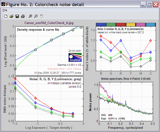
| The upper left plot is the density
response
of the
colorchecker (gray squares). It includes the first and second order
fits
(dashed blue and green
lines). The horizontal axis is Log Exposure (minus the target
density), printed on
the
back of the ColorChecker. Q-13 Stepchart provides a more detailed
density response curve. |
The upper right plot shows the noise in the
third colorchecker row, which contains the most strongly colored
patches: Blue, Green, Red, Yellow, Magenta, and Cyan. In certain
cameras noise may vary with the color. Problems may be apparent that
aren't visible in the gray patches.
|
| The lower left plot shows the R, G, B, and Y
(luminance) RMS noise for as a function of Log Exposure
each patch. RMS noise is expressed in f-stops, a relative measure that
corresponds closely to the workings of the human eye. This measurement
is described in detail in the Q-13
Stepchart tour. It is largest in the dark areas because the pixel
spacing between f-stops is smallest. |
The lower right region displays EXIF data, if
available. |
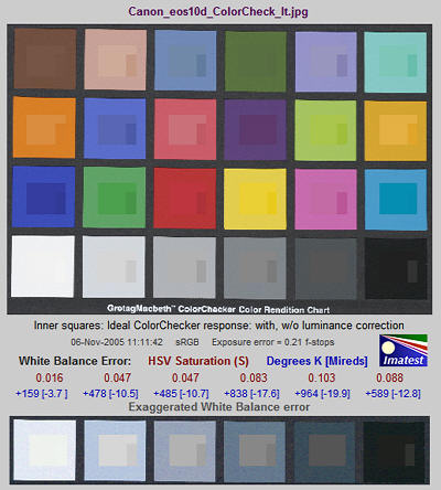
The third figure: color analysis
is an image of the ColorChecker with the correct colors superposed in the center
of each patch. The colors in the central squares are corrected for the
difference in luminance between the exposed and the ideal values. The colors
in the small rectangles to the right of central squares are uncorrected.
The gray patches with exaggerated White
Balance
error are shown on the bottom. White balance error is displayed in HSV
Saturation units, degrees Kelvin, and Mireds (1000/degrees K; a useful
unit for filtration).
|
|
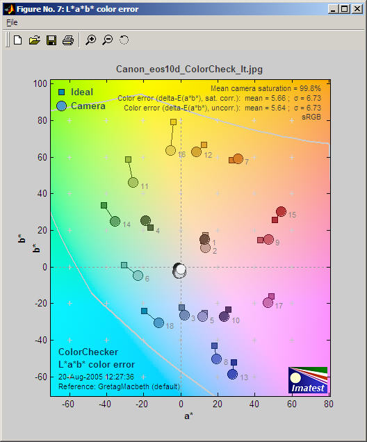
The fourth figure: color error
shows the color error
in the a*b* plane of the CIELAB color space, which is relatively perceptually
uniform (not perfect, but far more uniform than the common xy Chromaticity
diagram). The small squares are the ideal values; the large circles are
the measured (camera) values. The saturation of an individual color is
proportional to its distance from the origin (a* = b* = 0).
The mean camera
saturation (the average of all camera saturation values) relative to the
mean ideal saturation is displayed on the upper right, along with
the mean and RMS (root mean square) color error, measured with camera colors
corrected for saturation. The RMS error gives more weight to large errors.
Images can be analyzed in sRGB and Adobe RGB (1998)
color spaces.
|

|
|
|
Q-13 Stepchart
Measures tonal response, noise, and dynamic range using step charts
Q-13
Stepchart
Q-13
Stepchart
analyzes the tonal response, noise,
and dynamic range of digital
cameras and scanners using
Results are more detailed than those provided by Colorcheck. Transmission step charts are required for measuring dynamic range.
To run Q-13 Stepchart, load the image file, crop it (if needed), then specify the target density step (if different from the default value of 0.1 for reflective targets).
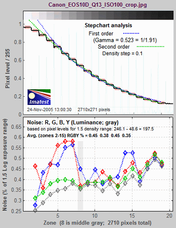
The two Figures below illustrate the results of analyzing a Q-13 image photographed with the Canon EOS-10D at ISO 100. |
 |
The first figure
contains basic tonal response and noise measurements.
The horizontal axis for both plots is the chart zone— proportional to the distance along the chart. Density (–Log Exposure) increases by a fixed step (0.10 or 0.15, depending on the target) for each zone.
The upper plot
shows the normalized pixel level of the
grayscale patches (black curve) and first and second order
density fits (dashed blue and green
curves). Gamma is derived from the first order fit.
The lower plot shows the RMS noise for each
patch:
for R, G, B, and Y (luminance) channels, expressed as the percentage of the range of
pixel levels corresponding to a target density range of 1.5: the same
as the white - black patches on the ColorChecker. The average noise for each channel (excluding the lightest and darkest zones) is displayed.
|
 |
The second
Figure
contains the
most important results:
- the response curve displayed on a log
scale, similar to film response curves,
- noise expressed in two
different ways (most meaningfully as a fraction of an f-stop or EV, explained below),
- dynamic range (for
transmission step charts),
- the noise spectrum.
The horizontal
axis for all three plots on the left is Log Exposure, which equals
(–) the nominal target
density
(0.05 - 1.95 for the Q-13/Q-14).
| The upper left plot shows the density response (gray squares), as well as the first and second order fits (dashed blue and green lines). It resembles a traditional film density response curve. Dynamic range is grayed out because the reflective Q-13 target has too small a dynamic range to measure a camera's total dynamic range. See Dynamic range, below. |
The upper right box contains dynamic range results: total dynamic range and range for several quality levels, based on luminance (Y) noise. It is shown in gray when a reflective target is selected. |

The middle left plot shows
noise in f-stops or EV, i.e., noise scaled to (divided by) the
difference in pixel levels between f-stops, which decreases as
brightness decreases. The darkest levels have the highest f-stop noise.
This
measurement corresponds to the response of the eye and has
important consequences for the calculation of practical dynamic range.
The vertical axis is logarithmic for clear display of low noise values.
|
EXIF data is shown in the
middle right region (JPEG files only).
|
The bottom left plot
shows the noise scaled to the difference in pixel levels between the
maximum density level and the patch corresponding to a density of 1.5—
the same density range as the GretagMacbeth Colorchecker. It may be less visually
meaningful then the middle plot.
|
The lower right plot
shows the noise
spectrum. Digital
camera images with excessive noise reduction will have an unusually
rapid
falloff of the noise spectrum. |
 Why measure noise in f-stops?
Because the human eye responds to
relative
luminance differences. That's why we think of exposure in terms of
zones, f-stops, or EV (exposure value),
where a change of one unit corresponds to halving or doubling
the exposure.
The eye's relative sensitivity is expressed by the Weber-Fechner
law,
ΔL ≈ 0.01 L –or– ΔL/L
≈ 0.01
where ΔL is the smallest luminance difference the eye can distinguish. (This equation is approximate; ΔL tends to be larger in dark areas of scenes due to visual interference from bright areas.)
Expressing noise in relative luminance units, such as f-stops, corresponds more closely to the eye's response than standard pixel or voltage units. Noise in f-stops is obtained by dividing the noise in pixels
by the number of pixels per
f-stop. (I use "f-stop" rather than "zone" or "EV" out of habit; any of them are OK.) |
noise in f-stops = noise in pixels / (d(pixel)/d(f-stop))
where d(pixel)/d(f-stop) is the derivative of the pixel level with respect to luminance measured in f-stops (~log2(luminance) ). |
|
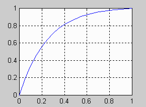
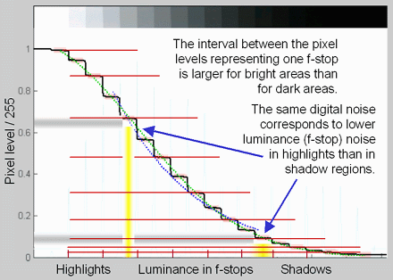
The above-right image illustrates how the pixel spacing between f-stops (and hence d(pixel)/d(f-stop))
decreases with decreasing brightness. This results in an increase of f-stop noise with brightness, visible in the middle-left plot of the second figure, above.
Because
luminance noise (measured in f-stops) is referenced to relative scene luminance,
independently of electronic processing or pixel levels, it is a universal measurement
that can be used to compare digital sensor quality.
|
Dynamic
range
Dynamic
range is the range of brightnesses over which a camera responds. It is
usually measured in f-stops, or equivalently, zones or EV. It can
be specified in two ways:
- The total range.
Q-13 Stepchart measures a camera's total dynamic range, including dark areas that may be extremely noisy.
- A range of tones over which the RMS noise, measured in f-stops, is under a maximum
specified value. The lower the maximum noise value, the better the
image
quality, but the smaller the dynamic range. Noise tends to be worst in
the darkest regions. Imatest calculates the
dynamic range for several maximum
noise levels, from RMS noise = 0.1 f-stop (high image
quality) to 1 f-stop (relatively low quality).
Dynamic
range is measured using transmission
step charts because they have density
ranges of at least 3.0: a 1000:1 ratio (10 f-stops), sufficient for
digital cameras. Reflective
charts such as
the
Q-13 have a density range of only around 1.90; an 80:1 ratio (6.3
f-stops).
The dynamic range is the difference in density between the zone where the pixel level is 98% of its maximum value (250 for 24-bit color, where the maximum is 255), estimated by interpolation, and the darkest zone that meets the measurement criterion. The repeatability of this measurement is better than 1/3 f-stop.
The
figure below illustrates results
for the Canon EOS-10D,
taken from a JPEG image acquired
at ISO 400 and converted with Canon Zoom Browser set for low contrast.
A Kodak step tablet (density from 0.05 to 3.05 in steps of 0.15) was
used.
The total dynamic
range is 8.6 f-stops. Total dynamic
range changes little for 48-bit TIFF conversion or ISO 100. But 48-bit
TIFF conversion has lower noise, hence higher dynamic range at any given
quality level.
Because the maximum noise is 0.44 f-stops (in the darkest
region), a medium quality image can be achieved when the full dynamic
range (8.6 f-stops) is utilized. When a high quality image is required (maximum noise = 0.1 f-stops),
the dynamic range is reduced to 6 f-stops (indicated by the yellow line on the middle left plot). High quality slide
film has a total dynamic range of 5 to 6 f-stops.
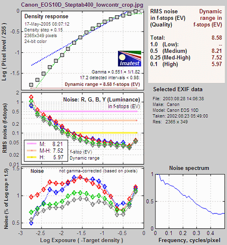
The
second plot contains all important Stepchart results.
The shape of the response curve
depends
strongly on the conversion software and settings.
Compact digital
cameras have much higher noise levels, hence lower useful dynamic
range, even though their total dynamic
range may be quite
large.
Scanner results
Here are the results of scanning the Kodak step
tablet with the Epson 3200 scanner set for negatives.

A few
observations on the scanner results:
- All 20 steps of the Kodak step tablet were detected. The total
dynamic range is greater than 3 density units (the 10 f-stop range
of the tablet). To determine the true total dynamic range we would need the Stouffer T4110 step wedge,
which has a maximum density of 4.
- The response closely follows an exponential curve with gamma =
0.506. No "S" curve has been superposed.
- The practical dynamic range is limited by noise. It is 9.62
f-stops (2.9 density units) for a medium quality image.
- The flat noise spectrum indicates that no software noise
reduction has been applied. Most digital cameras have rolloffs in their noise spectra due to Bayer interpolation and noise reduction.
SFR
Measures image sharpness using a slanted-edge target
SFR:
Measure sharpness
Imatest SFR
measures image
sharpness and several additional factors that contribute to image
quality,
including chromatic aberration, noise, and Shannon
capacity. It derives these results from a simple slanted-edge image, shown below. To measure sharpness,
Concise instructions for using Imatest SFR and interpreting its results can be found in How to test lenses with Imatest.
The primary sharpness indicator is MTF50, the spatial
frequency
where contrast drops to half its low frequency value.
Spatial Frequency Response (SFR), which is synonymous with Modulation Tansfer Function (MTF), is introduced in What
is image sharpness and how is it measured? The important section on Interpretation of MTF50 links MTF50 to print quality.
Sharpness
The Figure below illustrates the primary results of running Imatest
SFR. The two plots
display
sharpness results in two domains— spatial (the
average
edge profile) and frequency (the spatial frequency response (SFR/MTF) curves). They present
similar
information from two different viewpoints. Input data is shown
on
the right of the Figure: a thumbnail of the complete test image, the selected Region
of Interest (ROI), and selected EXIF data (information
recorded by the camera). The industry-standard ISO 12233 test chart is
shown, but you can print your own charts on a high
quality inkjet printer.

The upper left plot shows the
cross section
of an average edge. The narrower this edge, the better
the
performance. The black line is the orginal edge. The dashed
red line is the edge with standardized
sharpening— the output of an algorithm that sharpens (or
de-sharpens)
the image so the edge overshoot is similar for different cameras. This
allows
cameras with different amounts of built-in sharpening to be compared
fairly.
Standardized sharpening tones down the original edge of this particular camera, which is strongly
oversharpened.
The primary spatial domain performance indicator is the 10-90%
rise distance, indicated in black for the original
edge
and
red for the edge with
standardized
sharpening, labelled 10-90%(corr)
for "corrected." Shorter is better.
The lower left plot shows the Spatial Frequency
Response (SFR), also called modulation
transfer function (MTF), i.e., the image contrast
relative
to contrast at low spatial frequencies. Black is for the
original;
dashed
red is with standardized sharpening. The primary performance
indicator is MTF50 (the spatial
frequency
where image contrast drops to 0.5 = 50%). The higher the better, though
excessive
response above the Nyquist
frequency
(0.5 Cycles/Pixel; the highest spatial frequency where information can
be conveyed) may indicate aliasing problems (low frequency artifacts).
"Ideal megapixels" (shown in brackets [...] ) is the number of
megapixels with ideal response (MTF50 = 0.5 Cycles/Pixel) that would
have equivalent sharpness. Practical digital cameras rarely reach this
level; MTF50 around 0.33 Cycles/Pixel is very decent.
The
uncorrected response (MTF50 or 10-90% rise distance) is appropriate for
evaluating the performance of different lenses on a single digital
camera.
The response with standardized sharpening is appropriate for comparing
different digital cameras.
These measurements begin to make
sense when cameras
are compared, as they are here. The page on
Sharpness has more details on
MTF. SFR Results: MTF (sharpness) plot describes this Figure in detail.
Chromatic
aberration
Imatest measures lateral
chromatic aberration, also known as "color
fringing,"
which is most visible on tangential
boundaries near the edges of the image.
The curves for the R, G, and B color channels are shown
below. The visibility
of the chromatic aberration is proportional to the area
between the highest amplitude transition (in this case,
red)
and the lowest amplitude transition (in this case, blue).
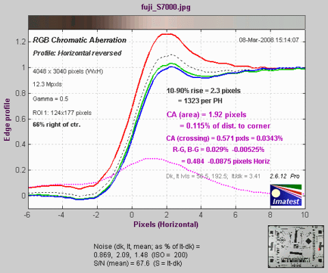
This area is called the
area chromatic aberration.
It is displayed in magenta. Since
the
edge amplitude is normalized to 1, area CA
can be measured in pixels— a
simple
unit of length. But since CA in pixels tends to be proportional to the distance from the image center, a better indication is obtained by expressing CA as the percentage of the distance from the image center. This has the advantage that it is relatively independent of the measurement location and the number of pixels in the camera. CA under 0.04% of the distance from the center is insignificant; CA over 0.15%
can be quite visible and serious. Much of the plot is grayed out if the selected region (ROI) is too close to the center (less than 30% of the distance to the corner) to accurately measure CA.
See Chromatic
Aberration for more details. Chromatic Aberration, Noise, and Shannon Capacity plot describes this Figure in detail.
Multiple
runs
Imatest SFR allows you to select
several regions of interest (ROIs) in a single run, then plot
performance
as a function of distance from the image center. A typical result is
shown
below.
The upper plot shows MTF50 without
and with standardized sharpening.
The
lower plot shows 10-90% rise distance and chromatic
aberration
(in pixels). The legend (lower right) can be moved with the mouse if it
covers data points. An MTF50 (sharpness) summary is displayed on the
right.
In calculating the Weighted MTF50, the image center is given twice the
weight of the corners. This number is an excellent indicator of overall
lens or camera sharpness.
Multiple ROI (Region of Interest) plot describes this Figure in detail.
Print test
Measures print quality factors: color response, tonal response, and Dmax
Introduction
Print test has been released as a beta version. A full release is planned for late November, when additional documentation is available.
Print test
measures several of the key factors that contribute to photographic print quality,
- color response, the relationship between pixels in the image file and colors in the print,
- tonal response, the relation between pixels and print density, and
- Dmax, the deepest printable black tone,
using a simple test pattern scanned on a flatbed scanner.
With Print test you can answer questions such as,
- What are the brightest colors my printer/paper/ink can make, i.e., what is its gamut?
- How dark a black tone can my printer/paper/ink make?
- How good are my ICC profiles? Do they provide smooth, uniform response? Are there instances where colors saturate? What are their specific strengths and weakness?
- How do colors map between color spaces and devices? What difference does rendering intent make?
Although the results are not as accurate in an absolute sense as those produced by expensive spectrophotometers, colorimeters, or densitometers, they are outstanding in a relative sense: for comparing prints made with different printers, inks, papers, and profiles. Absolute accuracy can be quite good in profiled scanners. You can see response irregularities with greater detail than with many of the more expensive instruments. And you can do so conveniently, using standard digital darkroom hardware.
Color quality is a function of gamut— the range of saturated colors a print can reproduce, as well as overall color response— the complex relationship between file pixels and hue, saturation, and lightness. Tonal quality is a function of Dmax— the deepest attainable black tone, as well as the tonal response curve. I've always regarded Dmax as particularly important: Prints appear weak to me if black tones aren't truly deep.Print test displays color gamut, color response, Dmax, and tonal response with unprecedented clarity and detail.
 Print quality depends on the
- printer,
- paper (manufacturer's or independent),
- ink (manufacturer's or independent),
- ICC profile,
- rendering intent (one of four rules, embedded in ICC profiles, for mapping pixels between color spaces or devices such as monitors and printers, and
- RIP (Raster Image Processor), an optional software package that is an alternative to standard printer drivers and profiles.
Even if you have only one printer, many options may be available. I use standard Epson Ultrachrome inks on my 2200 printer, but I can choose among a staggering variety of papers and profiles. And the often-overlooked profile rendering intent may make a difference.
The absolute accuracy of Print test results can be enhanced by calibrating the scanner with a standard target, such as the Kodak Q-13 Gray Scale and by measuring its response and creating an ICC profile using one of several available software packages.
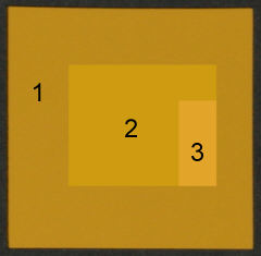
The test pattern, shown on the right, was generated using the HSL color representation.
- H = Hue varies from 0 to 1 for the color range R→ Y→ G→ C→ B→ M→ R (horizontally across the image on the right). (0 to 6 is used in some of the Figures below for clarity.)
- S = Saturation = max(R,G,B)/min(R,G,B).
- LHSL = Lightness = (max(R,G,B)+min(R,G,B))/2. (The HSL subscript is used to distinguish it from CIELAB L.)
The key zones are,
- S=1 square. A pattern consisting of all possible hues (0 ≤ H ≤ 1) and lightnesses (0 ≤LHSL≤ 1) in the HSL color representation, where all colors are fully saturated (S = 1), i.e., as saturated as they can be for the lightness value.
- L=0.5 rectangle. A pattern consisting of all possible hues (0 ≤ H ≤ 1) and saturation levels (0 ≤ S ≤ 1) for middle lightness (LHSL = 0.5), where the greatest saturation takes place.
- Two identical monochrome tone scales, where pixel levels vary linearly, 0 ≤ {R=G=B}≤ 1.
The zones labelled K, Gry, and W are uniform black (pixel level = 0), gray (pixel level = 127), and white (pixel level = 255), respectively.
Simplified instructions
 Download the Print test pattern, Print_test_target.png, which can also be found in the images subfolder of the Imatest installation folder. Download the Print test pattern, Print_test_target.png, which can also be found in the images subfolder of the Imatest installation folder. - Print the pattern, approximately 6.5x10 inches (16x25 cm), from your image editor, carefully recording the paper, ink, color space, ICC profile, and printer software settings.
- Scan the print on a flatbed scanner at 100-150 dpi. (Higher resolution is wasted; it merely slows the calculations.) The pattern must be aligned precisely (horizontally and vertically). If possible, the scanner's auto exposure should be turned off. If the scanner has an ICC Color Management setting, it should be used. It doesn't hurt to scan a Q-13 target next to the print. Save the scan with a descriptive name. TIFF, PNG, or maximum quality JPEG are the preferred formats. A reduced scan of a print made on the Epson 2200 printer with Epson Enhanced Matte paper and the standard Epson ICC profile is shown on the right. Colors are somewhat more subdued than glossy, semigloss, or luster papers.
- Run Q-13 Stepchart, using a Q-13 or equivalent reflective step chart. When the run is complete, check the box labelled "Save Print test calibration data" in the Save Q-13 Stepchart Results window. This saves the tonal response and Dmax calibration data, even if you click No to Save Q-13 Stepchart results? This only needs to be done once for a set of scans made under identical conditions. This step is optional. Print test doesn't require it, but it improves the accuracy of the tonal response and Dmax.
- Run Imatest. Select the Print test module. Crop the image so a small white border appears around the test pattern.
|
 |
Scanner color response: Because Print test results are filtered by the scanner's color response, it's a good idea to check it using Colorcheck. The response of the Epson 3200 with Epson's default ICC profile, shown on the right, is decent; comparable to the best digital cameras. If possible you should profile the scanner for best accuracy.
Print Test results are also filtered by the color space of the image file. Although no color space is embedded in the test image file, a color space is assumed when you make a print from an image editor. The default is sRGB, which has a limited gamut. You can select different color spaces if you have an ICC-compliant editor (Photoshop, Picture Window Pro, etc.). Adobe RGB (1998) is a good choice because it has a larger gamut than sRGB, but if you use it, be sure assign the Adobe RGB profile without changing the image pixels, i.e., do not perform a gamut mapping.
You should scan the image into the same color space you used to print it. Print test doesn't recognize embedded ICC profiles, but it allows you to select the color space manually.
|
Results
Results below are for Epson 2200 printer with Ultrachrome inks, Premium Luster paper, and the standard 1440 dpi Epson profile.
Density
The first Figure contains the grayscale density response and Dmax, the maximum density of the print, where density is defined as –log10(fraction of reflected light). The value of Dmax (2.04) is the average of the upper and right black areas.
The upper plot shows –print density as a function of log10(original pixel level (in the test pattern)/255). This corresponds to a standard density-log exposure characteristic curve for photographic papers. The blue plot is for the upper grayscale; the black plot is for the lower-right grayscale. Somewhat uneven illumination is evident. The print density values are calculated from Q-13 calibration curve (lower right). The thin dashed curves contain –log10(pixel levels).

The lower left curve is the characteristic curve (print vs. original normalized pixel level) on a linear scale.
The lower right curve is the results of the (separate) Q-13 calibration run used to calibrate Dmax and the density plot.
S=1 HSL Saturation map
The S=1 Figures are for region 1, which contains all possible hues (0 ≤ H ≤ 1) and lightnesses (0 ≤ LHSL ≤ 1) with maximum HSL saturation (S = 1).
The Saturation map shows the saturation levels. If the print and scanner response were perfect, S would equal 1 everywhere. Weak saturation is evident in light greens and magentas (L > 0.5). Strong saturation in darker regions, roughly 0.2 ≤ L ≤ 0.4, would seem to indicate that a better profile might perform better in the light green and magenta regions. Weak saturation in very light (L>0.95) and dark areas (L<0.1) is not very visible.

S=1 La*b* Gamut map
By transforming the S=1 Saturation map into the device-independent CIELAB color space, color gamut can be visualized in an entirely different way. In CIELAB, L is a nonlinear function of luminance (where luminance ≈ 0.30*Red + 0.59*Green + 0.11*Blue), a* represents colors ranging from cyan-green to magenta, and b* represents colors from blue to yellow. The colors of the a*b* plane are represented reasonably well in the background of the Figure below.
CIELAB is relatively perceptually uniform, meaning that the visible difference between colors is approximately proportional to the distance between them. It isn't perfect, but it's far better than HSL (where Y, C, and M occupy narrow bands) or or the familiar CIE 1931 xyY color space, where gamuts are represented as triangles or hexagons inside the familiar horseshoe curve. A CIE 1931 xyY Saturation map proved to be useless because of its perceptual nonuniformity: values bunched up along edges in a way that made results difficult to interpret. Note: The L-values below refer to LHSL in the test file, not CIELAB L.
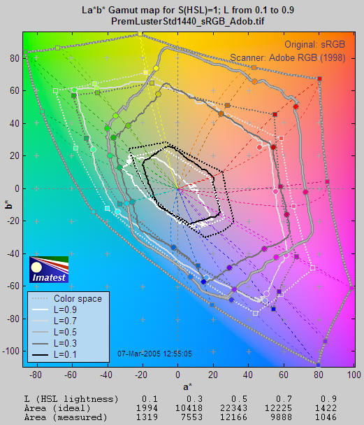
CIELAB color space is often displayed as a solid 3D volume. But although 3D displays can be visually impressive, they can be difficult to interpret. Print test displays an S=1 La*b* Gamut map as cross sections of the La*b* volume representing a*b* values for test file lightnesses (LHSL) of {0.1, 0.3, 0.5, 0.7, and 0.9}, corresponding to near black, dark gray, middle gray, light gray, and near white.
Although this display contains less information than the HSL map, but the results are clearer and more useful. The solid shapes from white to black) are the measured response for values of LHSL shown in the legend on the lower left. The dotted shapes represent the gamut of the color space (sRGB, in this case) at each LHSL level. CIELAB gamut varies with lightness: it is largest for middle tones (LHSL = 0.5) and drops to zero for pure white and black. This is closer to the workings of the human eye than HSL representation, where hues vary from 0 to 1, even for white and black.
The dotted concentric curves are the twelve loci of constant hue, representing the six primary hues (R, Y, G, C, B, M) and the six hues halfway between them.. They follow different curves above and below L = 0.5. The circles on the solid curves show the measured hues at locations corresponding to the twelve hue loci. Ideally they should be on the loci. The curves for L = 0.5 (middle gray) are outlined in dark gray to distinguish them from the background.
The hexagonal shape of the gamuts makes it easy to judge performance for each primary. The measured (solid) shape should be compared to the ideal (dotted) shape for each level. Weakness in magenta, blue, and green is very apparent, especially at L = 0.5 and L = 0.7. But the gamut is excellent for L = 0.3.
S=1 Lightness map
The ideal lightness map would display uniformly spaced horizontal lines from 0.9 near the top to 0.1 near the bottom. (It generally doesn't go much below 0.1 because of the effects of Dmax and gamma.This plot shows relatively uniform response except for blues with L between 0.3 and 0.6, which appear darker than they should.

S=1 Hue map
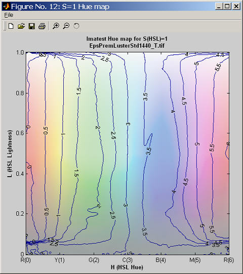
Colors are labelled 0 to 6, corresponding to hues from 0 to 1. This clarifies the plot by making each primary color an integer: Red = {0,6}, Yellow = 1, Green = 2, Cyan = 3, Blue = 4, and Magenta = 5. Contour increments are 0.5 instead of 0.08667. The ideal Hue map would consist of uniformly spaced vertical lines aligned with the x-axis. The hues here are rather good, but blues are a bit bloated and the magentas are somewhat squeezed. This is also visible on the S=1 Gamut map. There is a highly visible irregularity at L=0.6 on the blue-magenta border (also noticeable on the saturation map). Hue errors in very light (L>0.95) and dark areas (L<0.1) are not very visible.
Similar plots are produced for the L=0.5 region, immediately above the S=1 region.
L=0.5 HSL Saturation map
The L=0.5 Saturation map, which displays response to different levels of color saturation, is of interest for comparing different rendering intents (rules that control how colors are mapped when they are transformed between color spaces or color spaces and devices). Colorimetric rendering intents should leave saturation unchanged. Perceptual rendering intent expands color gamut when moving to a color space or device with increased gamut; it compresses it when moving to a smaller gamut. But there is no standard for perceptual rendering intent: every manufacturer does it in their own say. "Perceptual rendering intent" is a vague concept; it's hard to know its precise meaning unless you measure it.
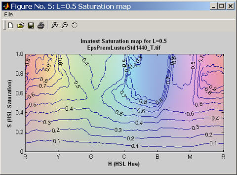
The ideal L=0.5 Saturation map would consist of uniformly spaced horizontal lines from 0.9 to 0.1. The weak saturation in the greens and magentas is visible here.
L=0.5 La*b* Gamut map
L=0.5 Saturation results become clearer when displayed on the CIELAB a*b* plane. Gamuts are shown for 0 ≤ S ≤ 1 in steps of 0.2. As in the the S=1 La*b* Saturation map, the dotted lines and shapes are the ideal values and the solid shapes are the measured values.
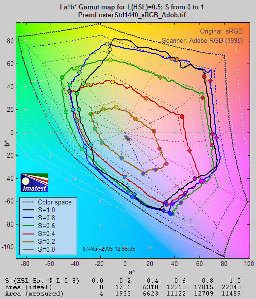
Gamut is excellent for S = 0.2 (brown) and 0.4 (red). But compression becomes apparent around S = 0.4 (red curve) for magenta and blue and S = 0.6 (green curve) for green and cyan, where the printer starts to saturate. Increasing S above these values doesn't increase the print saturation: in fact, saturation decreases slightly at S = 1. This is the result of limitations of the Epson 2200's pigment-based inks and the workings of the standard Epson ICC profile.
With Gamut maps, differences between printers, papers, and profiles are immediately apparent. These differences are far more difficult to visualize without Imatest Print test because each image has its own color gamut. One image may look beautiful but another may be distorted by the printer's limitations.
An additional Figure with L=0.5 Hue and Lightness maps has been omitted.
Sharpness
What is it and how is it measured?
Image sharpness
Photographic image sharpness is defined by the boundaries between
zones
of different tones or colors. It is illustrated by the bar pattern of
increasing
spatial frequency, below. The top portion represents a target used to
test
a camera/lens combination. It is sharp;
its boundaries are abrupt, not gradual. The bottom portion illustrates
the effect of a high quality 35mm lens on a 0.5 millimeter long image
of
the pattern (on the film or digital sensor plane). It is blurred.
All lenses, even the finest, blur the image to some degree. Poor lenses
blur the image more than fine ones.

One way to measure sharpness is to use the rise
distance of the edge, for example, the distance (in pixels
or millimeters) for the pixel level to go from 10% to 90% of its final
value. This is called the 10-90% rise distance. Although rise distance
is a good indicator of image sharpness, it has one limitation. It is
poorly suited for calculating the sharpness of a complete imaging
system
from the sharpness of its components, for example, from a lens, digital
sensor, and sharpening algorithm.
To get around this problem, measurements are made in frequency
domain, where frequency is measured in cycles
or line pairs per distance
(typically millimeters, but sometimes inches). Line
pairs per millimeter (lp/mm)
is the most common spatial frequency unit. The
image below is a sine wave— a pattern of pure tones— that varies from
low to high spatial frequencies, in this case from 2 to 200 lp/mm, over
a distance of 0.5 millimeters. The top portion is the
original
sine pattern. The bottom portion illustrates the effects of the same
high
quality 35mm lens, which reduces pattern contrast at high
spatial frequencies.
The relative contrast at a given spatial frequency (output
contrast/input contrast) is called the Modulation Transfer
Function (MTF) or Spatial Frequency Response (SFR).
Illustration of Modulation
Transfer Function (MTF)
(Spatial frequency response (SFR) )
|
The upper plot displays the sine and bar patterns: original
and after blurring by the lens.
The middle plot displays the luminance of the bar pattern after
blurring
by the lens (the red curve).
Contrast
decreases at high spatial frequencies.
The lower plot displays the corresponding MTF (SFR) curve (the
blue curve).
By definition, low frequency MTF is always 1 (100%). For this lens,
MTF is 50% at 61 lp/mm and 10% at 183 lp/mm.
Both frequency and MTF are displayed on logarithmic scales with
exponential
notation (100 = 1; 101 = 10; 102 = 100,
etc.). Amplitude is displayed on a linear scale.
The beauty of using MTF is that the MTF (i.e., Spatial Frequency
Response)
of a complete imaging system is the product of the the MTF of its
individual
components.
|
 |
Green is
for geeks. Do you
get excited by a good equation? Were you passionate about your college
math classes? Then you're probably a math geek— a member of a maligned
and misunderstood but highly elite fellowship. The text in green is for
you. If you're normal or mathematically challenged, you may skip these
sections. You'll never know what you missed.
MTF is related to edge response by a mathematical
operation known as the
Fourier transform.
MTF is the Fourier
transform of the impulse response— the response to a narrow line,
which
is the derivative (d/dx) of the edge response. Fortunately, you don't
need
to understand Fourier transforms or calculus to understand MTF.
Traditional "resolution" measurements involve observing an image of
a bar pattern (usually the USAF 1951 chart) on film, and looking for
the
highest spatial frequency (in lp/mm) where a pattern is visible. This
corrresponds
to an MTF of about 2-5%. Because this is the spatial frequency where
image
information disappears— where it isn't
visible, it is not a good indicator of image sharpness.
Experience has shown that the
best indicator of image sharpness is the spatial frequency where MTF is
50% of its low frequency value
(MTF50).
MTF50 is an ideal parameter for comparing the sharpness of different
cameras
for several reasons: (1) Image contrast is half its low frequency
value,
hence detail is still quite visible. (2) The eye is relatively
insensitive
to detail at spatial frequencies where MTF is low: 10% or less. (3) The
response of virtually all cameras falls off rapidly in the vicinity of
MTF50.
 Although
MTF can be estimated from images of a sine pattern (see the page on Lens testing),
a sophisticated technique, based on the ISO
12233:2000 standard, "Photography - Electronic still picture
cameras
- Resolution measurements," yields more accurate, repeatable
results.
A slanted-edge image, described below, is photographed, then analyzed
by
the Imatest SFR program. (SFR
stands for Spatial Frequency Response.)
The algorithms for calculating MTF/SFR in Imatest SFR were adapted
from
a Matlab program, sfrmat, written by Peter Burns to implement the ISO
12233
standard. The original code is available on the I3A
download page on ISO
12233
Slant Edge Analysis Tool sfrmat 2.0. You can write Peter at  .
.
The slanted-edge test for Spatial Frequency Response
A typical portion is shown on the right: a crop of a vertical edge (slanted about 5.6 degrees), used to calculate horizontal MTF response. An advantage of the slanted edge test is that the camera-to-target distance isn't critical. It doesn't enter into the equation that converts the image into MTF response.
For the mathematically-minded, here are the details of the calculations. The cropped image is entered into a program that linearizes the levels (correcting for an assumed gamma of 2), then determines the average edge location of the luminance channel (Y = 0.3*Red + 0.59*Green + 0.11*Blue). The edge profile of each line is added to one of four bins that to calculate an averaged 4x oversampled edge. This allows analysis of spatial frequencies beyond normal limits. MTF is the absolute value of the Fourier transform (FFT) of the windowed derivative of the averaged edge. |

|
Imatest SFR results
35mm camera lens tests use line
pairs per millimeter (lp/mm) as the
units of spatial frequency. This works fine for comparing lenses
because
all 35mm cameras have the same 24 mm picture height. But sensor height in digital
varies widely, from less than 5 mm in
ultra-compact
models to 24 mm for full-frame DSLRs; even larger for medium format
backs.
The number of pixels also varies. For this reason, a measure of spatial
frequency is needed that indicates the total
response rather than the response per distance.
For this purpose we use line widths per picture height
(LW/PH)
as a spatial frequency unit for digital cameras. LW/PH is equal to 2
* lp/mm * (picture height in mm). Where total
picture height is involved, line widths is
customarily used instead of pairs (where one line pair
equals two line widths).
The use of picture height gives a slight advantage
to compact digital cameras, which have an aspect ratio (width:height)
of
4:3, compared to 3:2 for digital SLRs. Compact digital cameras have
slightly
more vertical pixels for a given number of total pixels. For example, a
5.33 megapixel compact digital camera would have 2000 vertical pixels—
as many as a 6 megapixel DSLR.
Another measure of spatial frequency used
with digital cameras is cycles
or line pairs
per pixel
(c/p
or lp/p).
This gives an indication of how well individual pixels are being
utilized.
There is no need to use actual distances (millimeters or inches) to
evaluate
digital camera image quality, although such measurements are an available option in Imatest SFR.
Imatest SFR program output contains results on the left and input data on the right (a
thumbnail of the entire image, the region of interest (ROI), and
selected EXIF data).
|
(top) A narrow image that illustrates the tones of the
averaged
edge. It is aligned with the edge profile (spatial domain) plot,
immediately
below.
(middle) Spatial
domain plot: The average edge profile. The key result is the 10-90%
edge rise distance, shown in pixels and in the
number of rise distances per picture height. The
red values are for standardized
sharpening. Other parameters include overshoot and undershoot (if applicable).
(bottom) Frequency
domain plot: The Spatial Frequency Response
(MTF), shown to twice the Nyquist
frequency. The key result is MTF50,
the 50% MTF frequency, which corresponds to perceived image sharpness.
It is given in cycles per pixel (c/p) and line widths per picture
height
(LW/PH). Other results include MTF
at NYQ, the MTF at the Nyquist frequency (0.5
cycles/pixel; sampling rate/2), which indicates the probable severity of aliasing. The
Nyquist
frequency is displayed as a vertical blue line.
|
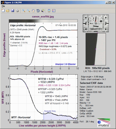
Results from the ISO 1233 image for the Canon EOS-10D. |
SFR Results: MTF (sharpness) plot describes this Figure in detail.
Interpreting MTF50
What MTF50 do you need? It depends on print size. If you plan to print gigantic posters (20x30 inches or over), the more the merrier. Any high quality 4+ megapixel digital camera (one that produces good test results; MTF50(corr) > 0.3 cycles/pixel) is capable of producing excellent 8.5x11 inch (letter-size; A4) prints. At that size a fine DSLR wouldn't offer a large advantage in MTF. With fine lenses and careful technique (a different RAW converter from Canon's and a little extra sharpening), my 6.3 megapixel Canon EOS-10D (corrected MTF50 = 1340 LW/PH) makes outstanding 12x18 inch prints. Prints are razor sharp from normal viewing distances, but pixels are visible under a magnifier or loupe; the prints are not as sharp as the Epson 2200 printer is capable of producing. Softness or pixellation would be visible on 16x24 inch enlargements. Sharpness comparisons contains tables, derived from images downloaded from two well-known websites, that compare a number of digital cameras. Several outperform the 10D.
The table below is an approximate guide to quality requirements. The equation for the left column is
| MTF50(Line Widths / inch on the print) = |
MTF50(LW/PH)
Print height in inches |
MTF50 in
Line Widths/inch
on the print |
Quality level— after post-processing, which may include some additional sharpening |
| 150 |
Excellent— Extremely sharp at any viewing distance. About as sharp as most inkjet printers can print. |
| 110 |
Very good— Large prints (A3 or 13x19 inch) look excellent, though they won't look perfect under a magnifier. Small prints still look very good. |
| 80 |
Good— Large prints look OK when viewed from normal distances, but somewhat soft when examined closely. Small prints look soft— adequate, perhaps, for the "average" consumer, but definitely not "crisp.". |
Example of using the table: My Canon EOS-10D has MTF50 = 1335 LW/PH (corrected; with standardized sharpening). When I make a 12.3 inch high print on 13x19 inch paper, MTF50 is 1335/12.3 = 108 LW/in: "very good" quality; fine for a print that size. Prints look excellent at normal viewing distances for a print this size.
This approach is more accurate than tables based on pixel count (PPI) alone. Pixel count is scaled differently; the numbers are around double the MTF50 numbers. The EOS-10D has 2048/12.3 = 167 pixels per inch (PPI) at this magnification. This table should not be taken as gospel: itwas first published in October 2004, andit may be adjusted in the future.
Some observations on sharpness
- Frequency and spatial domain plots convey similar information,
but in a
different form. A narrow edge in spatial domain corresponds to a broad
spectrum in frequency domain (extended frequency response), and
vice-versa.
- Response above the Nyquist frequency is garbage— aliasing,
visible as
Moire patterns of low spatial frequency. In Bayer sensors (in all
sensors
except Foveon) Moire patterns appear as color fringes. Moire in Foveon sensors is far less bothersome because it's monochrome.
- Results are for the Luminance (Y) channel, where Y = 0.3*R
+ 0.6*G + 0.1*B. Separate R,
G, and B results can be calculated if needed.
- Horizontal and vertical resoluton can be different for CCD
sensors, and
must be measured separately. They're nearly identical for CMOS sensors.
Recall, horizontal resolution is measured with a vertical edge and
vertical
resolution is measured with a horizontal edge.
- Resolution is not the only important criterion for evaluating
image
quality.
Noise is nearly as important. The Shannon
information capacity is a metric that combines the two.
The
ideal response would have high MTF below
the Nyquist frequency and low MTF at and above it.
Links
This
page has some interesting material on Fuji sensors and the history
of the slanted-edge test.
Spatial
Frequency
Response of Color Image Sensors: Bayer Color Filters and Foveon X3
by Paul M. Hubel, John Liu and Rudolph J. Guttosch, Foveon, Inc., Santa
Clara, California. Uses slanted edge testing.
Sharpening
Why standardized sharpening is needed for comparing cameras
Introduction to sharpening
Sharpening is an important part of digital image
processing. It restores some of the sharpness lost in the
lens
and the sensor chip. Virtually every digitized
image
is sharpened at some point in its workflow— in the camera, the
RAW conversion software, the image editor, or "all of the above."
Almost every digital camera sharpens images to
some degree. The problem is that each manufacturer and each model has
its
own sharpening algorithm. Some models sharpen images more than others—
sometimes more than appropriate. This makes it difficult to
determine
a camera's intrinsic sharpness. Imatest has developed a solution to
the
problem— standardized sharpening.
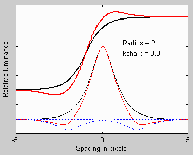
Before we proceed, we need to describe the elementary
sharpening process..
A simple sharpening algorithm subtracts a fraction of two
neighboring
pixels from each pixel, as illustrated on the right. The thin
black curve is the input to the sharpening function: it is the
camera's response to
a point or sharp line (called the line or point
spread function or impulse response).
The two thin dashed blue curves are
replicas of the input multiplied by -ksharp/2 and shifted by a distance of
±2 pixels (typical of the sharpening applied to digital
cameras). This distance is called the sharpening radius. The
thin
red
curve the impulse response after sharpening— the sum of the black
curve and the two blue curves. The
thick black and red curves (shifted
up and left) are the corresponding edge responses,
unsharpened and sharpened.
Sharpening increases image contrast at boundaries by reducing the rise distance. It
also
causes an edge overshoot (a small overshoot in this illustration).
Small
overshoots
enhance the perception of sharpness, but large overshoots, known as "halos," can become
glaringly
obvious, and can detract from image quality.
Sharpening also boosts
MTF50
(the 50% MTF frequency, which is an indicator of perceived sharpness—
a good thing) and it boosts noise (not so good). Virtually all digital
images
benefit
from the right amount of sharpening.
The formula for the simple
sharpening algorithm is,
Lsharp(x) = (L(x) - ksharp/2*(L(x-V) + L(x+V)) / (1-ksharp)
L(
x) is the input pixel level and L
sharp(
x)
is the sharpened
pixel level. Ksharp is the sharpening constant (related to the slider
setting
scanning or editing program). V is the shift used for sharpening.
V
= R/dscan, where
R is the sharpening radius (the
number
of pixels between original image and shifted replicas) in pixels.
1/dscan
is the spacing between pixels.
The sharpening algorithm has its own MTF (the Fourier transform of L
sharp(
x)).
MTFsharp(f) = (1-ksharp*cos(2*pi*f*V))/(1-ksharp)
This equation boosts response at high spatial frequencies. Maximum
boost takes place
where cos(2*pi*
f*
V
) = cos(pi) = -1, or
f = 1/(2*
V)
= dscan/(2*
R). This is equal to the Nyquist frequency,..
fN
=
dscan/2, for
R = 1 and lower for
R > 1.
Actual sharpening
is a
two dimensional operation.
Standardized sharpening
The degree of sharpening performed by digital cameras
varies greatly.Some cameras and many RAW converters allow you to change
the amount of sharpening from the default value. If an image is
undersharpened,
the photographer will need to apply additional sharpening during the
image
editing process for best results. Many compact digital cameras oversharpen
images, resulting in severe peaks or "halos" near boundaries. This
makes
small prints (4x6 or 5x7
inches) look good straight out of the camera, but it doesn't truly
enhance
image quality: halos can get ugly in big enlargements and noise can
become
objectionable.
Sharpening increases the 50% MTF frequency
(MTF50).
A camera with extreme oversharpening may have an impressive MTF50 but
poor
image quality. A camera with little sharpening will have an MTF50 that
doesn't
indicate its potential. For these reasons, comparisons
between cameras based on simple MTF50 measurements have little meaning.
Raw MTF50 is a poor measure of a camera's intrinsic sharpness,
even though it correlates
strongly with perceived image sharpness.
To obtain a good measure of a camera's sharpness— to compare
different
cameras on a fair basis, the differences in sharpening must be removed
from the analysis. The best way to accomplish this is to set the
sharpening
of all cameras to a standard amount.
This means sharpening undersharpened images and de-sharpening
(blurring)
oversharpened images.
The algorithm for standardized sharpening takes advantage of the
observation
that most digital cameras sharpen with a radius of about 2 pixels. This
has been the case for most of the cameras I've analyzed using data from dpreview.com
and imaging-resource.com.
The algorithm for standardized sharpening is as follows.
1. Apply sharpening (or de-sharpening) with a radius
of 2 to make the
MTF at 0.3 times the
Nyquist
frequency (0.3
x fN =
0.15
xdscan;
a relatively low spatial frequency) equal to 1 (100%), the same MTF as
very low spatial frequencies. MTF at higher spatial frequencies falls
where
it will, depending on lens and imager quality. The sharpening radius is adjustable in Imatest; 2 is the default.
2. Linearize the phase of the pulse by removing the imaginary part of the MTF. This results in an
antisymmetrical
pulse.
The resulting pulse has a small overshoot (halo) near edges—
typical
of what you would get with carefully-done manual sharpening.
If the edge is seriously blurred, so that there is very little
energy
at 0.3
x fN (MTF50 <
0.2
xfN
), the sharpening radius is increased and the equalization
frequency is decreased
to 0.6
* MTF50.
The formula for standardized
sharpening with radius
R (= 2) is,
MTFstandard(f) = MTF( f ) x (1-ksharpxcos(4xpixRxf/dscan))/(1-ksharp)
where sharpening constant ksharp is set so MTF
standard(0.3
fN
) = MTF(0) = 1.
fN =
dscan/2
is the
Nyquist
frequency.
The image is sharpened if ksharp > 0 and de-sharpened (ksharp
< 0; a bit
different from standard blurring) if ksharp < 0. For
R = 2,
the
maximum change takes place at half the Nyquist frequency,
f = fN
/2
= dscan/4, where cos(4*pi*
R*
f /dscan) =
cos(pi)
= -1. Sharpening with
R = 2 has no effect on the response at
the
Nyquist frequency because cos(4*pi*
fN
/dscan) = cos(2*pi) = 0.
Raw MTF50, without standardized sharpening, produces more accurate
results
for comparing the sharpness of different lenses, focal lengths, and
apertures
on one camera, as well as for comparing the sharpness at the center and
edge of a single image. But standardized sharpening is superb for
comparing
different cameras.
Examples
|
|
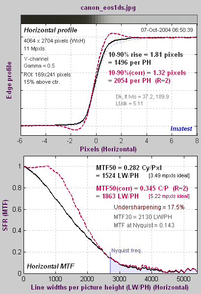
An undersharpened image
The 11 megapixel Canon
EOS-1Ds DSLR
is unusual in that it has very little built-in sharpening (at least in this particular sample).
The average edge (with no overshoot)
is shown on top; the MTF response is shown on bottom. The black
curves are the original, uncorrected data; the dashed red curves have standardized sharpening applied.
Standardized sharpening results in a small overshoot in the spatial
domain
edge response, about what would be expected in a properly sharpened
image. It is relatively consistent for all cameras. |
Oversharpening or undersharpening is the degree to which the uncorrected pulse is over- or undersharpened, i.e., sharpened relative to the standard sharpening
value.
It is equal to (-)ksharp in the above equation. It if is negative (the
case for the EOS-1Ds), sharpening is applied to the original response;
if it is positive, de-sharpening is applied. (I use "de-sharpening"
instead
of "blurring" because the inverse of sharpening is, which applied here,
is different from conventional blurring.) Note that it is not
the actual sharpening applied by the camera and software.
|

|
An oversharpened image
The image to the right is for the 5 megapixel Canon G5, which
strongly oversharpens the image— typical for a compact digital camera.
The uncorrected 10-90% edge rise distance of the G5 is
considerably
better than the 11 megapixel EOS-1Ds (1940 vs. 1511 per PH), but the
corrected
10-90% rise (with standard sharpening) is 76% of the EOS-1Ds. Based on
pixels alone, the expected percentage ratio would be 100% (1944/2704) =
72%. |
The raw MTF50 of the G5 is close to the EOS-1Ds, but the corrected
MTF50
(with standard sharpening) is 73% of the EOS-1Ds, very close to the
ratio
of vertical pixels.
These results illustrate how uncorrected rise distances and MTF50s
can
be extremely misleading when comparing cameras with different pixel
sizes
and degrees of sharpening. Uncorrected MTF50 is, however, appropriate
when
comparing different lenses, focal lengths and apertures on a single
camera.
Sharpness comparisons
for several digital cameras
Sharpness results derived from Websites
Several websites publish images of ISO 12233 test charts that can be entered into Imatest SFR to obtain detailed sharpness measurements. This page contains sharpness results derived from charts downloaded from two sites:
Two areas, delimited by red rectangles, are used for the measurements.
- First row: near the center. The rectangle just above the center of the chart (about 15% of the distance to the corners).
- Second row: near the corner. The rectangle in the lower right of the chart (about 78% of the distance to the corner). Results include Chromatic aberration, which cannot be measured near the center.

These measurements are limited to
- One lens. For DSLRs this is usually one of the sharpest available, such as the 50mm f/1.4 prime (non-zoom).
- One focal length. Sharpness is a strong function of focal length for zoom lenses. The sites aren't very consistent in their choice of focal length; long, short or intermediate focal lengths may be chosen.
- One aperture, typically around the optimum: f/8-f/11 for DSLRs; f/4-f/5.6 for compact digital cameras.
- One ISO speed, which has a stronger effect on noise and dynamic range than on sharpness.
- One RAW converter (usually the JPEG converter built into the camera) with one setting, usually the default settings. The choce of converter and sharpness setting has a strong effect on sharpness measurements.
- Gamma assumed to be 0.5, typical for digital cameras. SFR results are somewhat sensitive to the gamma estimate: a 10% gamma error results in a 2.5% MTF50 error. For greatest accuracy, gamma should be measured with Q-13 Stepchart or Colorcheck.
- The lighting isn't always optimum: if it is too dim or bright there can be some clipping on data (where it goes pure black or white), which affects sharpness measurement accuracy.
If you want to compare your own camera or lenses with the published charts, test lenses at various focal lengths and apertures, or observe the effects of ISO speed and signal processing, you'll need to download Imatest. The trial version allows up to twenty runs.
Explanation of results
| Megapixels |
The total megapixel count for the camera. |
| Picture
height
pixels |
The picture height of the camera. Important because sharpness is measured in units of Edge Rises or Line Widths per Picture Height. |
| Oversharpening % |
The amount of sharpening relative to standardized sharpening, which results in a modest amount of overshoot, similar to what you might get after a manual sharpening operation. Undersharpening (as reported in Imatest SFR) is displayed here as a negative number. |
| 10-90%
rises per PH
(raw) |
The number of intervals per Picture Height where the average edge signal (with gamma removed) rises from 10% to 90% of its final value. The more the better, though aliasing can be a problem for extremely high values (significantly larger than the picture height), especially with Bayer sensors. See Understanding sharpness and SFR tour. |
| 10-90%
rises per PH (corr.) |
The number of 10% to 90% rise intervals per Picture height after standardized sharpening. This allows cameras with different degrees of sharpening to be compared on a (relatively) fair basis. |
MTF50
LW/PH
(raw) |
The spatial frequency where contrast drops to half its low frequency value. This is the best indicator of sharpness. See Understanding sharpness and SFR tour. |
MTF50
LW/PH
(corr.) |
MTF50 with standardized sharpening applied (corrected). MTF50 with standardized sharpening is best for comparing cameras with different amounts of sharpening; MTF50 without standardized sharpening (uncorrected) is best for testing and comparing lenses on a single camera model. |
| Chromatic aberration (CA) |
A measure of "color fringing" near the edges of the images. Units are pixels. Tends to increase linearly with the distance from the center of the image. Under 0.5 pixels is insignificant. Over 1.5 is severe: quite visible in large prints. See Chromatic Aberration. An improved CA measurement, percentage of distance from the image center, is being implemented. |
Shannon
capacity
MB |
The information capacity of the image, based on sharpness (with standardized sharpnening) and noise. It correlates well with perceived image quality. But it should be interpreted with caution because it is strongly affected by signal processing, especially noise reduction. Best when used with RAW files. The number below is for a signal with the same contrast (100%) as the target (around 80:1). Shannon capacity is a relatively new measurement. We are still learning how to interpret it. |
| Comments |
Contains the source of the image (DPR or IR), and, if available, the focal length, aperture, and ISO speed. |
Tables of results
DSLRs: Digital SLRs, which take interchangeable lenses. Used by professionals and serious amateurs. Minimum sensor size is 22 mm diagonal. Larger and heavier than the compact digital cameras, below. This table is more complete than the table for compact digitals because it's where my interest lies.
| Camera |
Mega-
pixels |
Over-
sharp-
ening % |
10-90%
rises/PH
(raw) |
10-90%
rises/PH
(corr.) |
MTF50
LW/PH
(raw) |
MTF50
LW/PH
(corr.) |
Chro-
matic
Aber-
ration |
Shannon
capacity
MB |
Comments |
Picture
height
pixels |
| Canon EOS-1D Mk II |
8.2 |
-15 |
1351 |
1741 |
1355 |
1559 |
— |
5.56 |
DPR. 50mm f/9 ISO 100. Very little built-in sharpening. Optimized for speed. Same pixel count as EOS-20D, but larger pixels. |
| 2336
| -21 |
1178 |
1589 |
1173 |
1443 |
0.40 |
4.99 |
| Canon EOS-1Ds |
11 |
-17 |
1509 |
2045 |
1521 |
1860 |
— |
7.11 |
DPR. 100mm f/9 ISO 100. Little, if any, built-in sharpening. |
| 2704 |
-17 |
1485 |
2016 |
1519 |
1852 |
0.30 |
7.06 |
| Canon EOS-10D |
6.3 |
0 |
1419 |
1508 |
1332 |
1335 |
— |
4.02 |
DPR. 50mm f/9 ISO 100. Nearly identical to
the EOS-300D. My own camera and standard of comparison. Makes excellent
13x19 inch prints. |
| 2048 |
-1 |
1410 |
1480 |
1331 |
1339 |
0.55 |
3.95 |
| Canon EOS-20D |
8.2 |
8 |
1850 |
1778 |
1627 |
1581 |
— |
5.44 |
DPR. 50mm f/9 ISO 100. Successor to the EOS-10D. |
| 2336 |
3 |
1872 |
1789 |
1681 |
1664 |
0.58 |
5.82 |
| Fuji S2 Pro |
6/12* |
-12 |
1869 |
2104 |
1819 |
1832 |
— |
7.19 |
DPR. 50mm f/9.5 ISO 100. *SuperCCD diagonal
pixel array. Uses interpolation to increase pixel count. Unusual ringing
in edge. High noise reduction? |
| 2848 |
-7 |
1699 |
1987 |
1708 |
1756 |
0.73 |
6.72 |
| Kodak SLR/c |
14 |
7 |
3571 |
3457 |
3184 |
3177 |
— |
15.1 |
DPR. No anti-aliasing filter.
Exceptional sharpness, but has problems with color Moire, illustrated
here. (MTF > 0.5 at Nyquist.)
Strong noise reduction evident in the noise spectrum. Canon mount. The SLR/n is similar, but a Nikon mount. *CA is double the measured value for the half-size (2250x1500) image, using the observation that CA is proportional to distance from the lens center. |
| 3000 |
6 |
3619 |
3436 |
3202 |
3195 |
1.1* |
15.4 |
| Nikon D100 |
6 |
-3 |
1381 |
1437 |
1243 |
1262 |
— |
3.44 |
DPR. 50mm f/'9. Competitive with the
Canon EOS-10D. |
| 2000 |
-4 |
1300 |
1373 |
1186 |
1227 |
0.74 |
3.3 |
| Nikon D70 |
6 |
5 |
1590 |
1897 |
1766 |
1759 |
— |
4.72 |
DPR. 50mm f/9. Less aggresive anti-aliasing
filter than theD100. Excellent sharpness for the pixel count. Relatively high MTF at Nyquist (0.4). |
| 2000 |
4 |
1769 |
1849 |
1700 |
1688 |
0.71 |
4.61 |
| Olympus E1 |
5 |
-8 |
1174 |
1351 |
1142 |
1215 |
— |
2.89 |
DPR. 50mm f/5 ISO 100. (Wider than optimum aperture) 4/3" format. Curious spikes in noise spectrum at quarter multiples of Nyquist. Otherwise relatively flat noise spectrum indicates little noise reduction. |
| 1920 |
-10 |
1121 |
1325 |
1105 |
1201 |
0.21 |
2.86 |
| Sigma SD10 |
3.4 |
-2 |
1574 |
1618 |
1508 |
1508 |
— |
3.53 |
DPR. 50mm f/9 ISO 100. Foveon sensor: no
Bayer array. Apparently no anti-aliasing filter. Outstanding sharpness for the nunber
of pixels (if only it had more!) Very high MTF at Nyquist
(0.5), but little apparent problem with Moire. See this report. |
| 1512 |
-2 |
1463 |
1487 |
1381 |
1383 |
1.0 |
3.18 |
Compact digital cameras: These are primarily consumer cameras, though many produce excellent image quality, especially for letter-size or A4 prints. Most have non-interchangeable zoom lenses. Maximum sensor size is 11 mm diagonal.
| Camera |
Mega-
pixels |
Over-
sharp-
ening % |
10-90%
rises/PH
(raw) |
10-90%
rises/PH
(corr.) |
MTF50
LW/PH
(raw) |
MTF50
LW/PH
(corr.) |
Chro-
matic
Aber-
ration |
Shannon
capacity
MB |
Comments |
Picture
height
pixels |
| Canon G3 |
4 |
18 |
1636 |
1360 |
1265 |
1157 |
— |
2.19 |
DPR. 17.6mm f/4.5. Oversharpened. |
| 1704 |
11 |
1346 |
1186 |
1134 |
1052 |
1.27 |
|
| Canon G5 |
5 |
20 |
1931 |
1565 |
1458 |
1346 |
— |
2.88 |
DPR. 14.4mm f/4.0. Oversharpened. The chromatic aberration is not quite as bad as indicated because R and G are together; only B, to which the eye is less sensitive, is separate. |
| 1944 |
12 |
1774 |
1544 |
1399 |
1327 |
1.81 |
2.78 |
| Canon G6 |
7 |
12 |
2024 |
1780 |
1707 |
1612 |
— |
4.39 |
DPR. 15.2mm f/5.0. |
| 2304 |
-1 |
1738 |
1726 |
1599 |
1606 |
0.9 |
4.24 |
Fuji
F810 |
12.3* |
13 |
2085 |
1962 |
1944 |
1791 |
— |
6.02 |
DPR. 15.1mm f/5.6 ISO 80. *SuperCCD diagonal pixel array. Pixels are doubled in the test image. The lens is much better at the edges than the S7000. |
| 3040 |
-6 |
1906 |
1937 |
1829 |
1762 |
2.19 |
5.87 |
Fuji S7000
UL
LR |
6/12* |
22
|
2014
|
1853
|
1912
|
1625
|
—
|
5.21
|
DPR. 13mm f/5.6 ISO 200 (a high ISO speed for a compact; somewhat noisy). Oversharpened. *SuperCCD diagonal pixel array; 6 megapixels orig; 12 used for measurement. Uses interpolation to increase pixel count. UL = upper left; LR = lower right (the usual) ROIs. Softness on the left was noted by dpreview.com. Edge falloff is considerable. |
| 3040 |
-17
-22 |
1137
1202 |
1567
1591 |
1241
1230 |
1388
1446 |
2.67
2.04
|
4.52
4.62
|
Konica-Minolta
DiMAGE A2 |
8 |
8 |
1829 |
1696 |
1611 |
1537 |
— |
4.71 |
DPR. 13.3mm f/5.0 ISO 64. |
| 2448 |
-3 |
1500 |
1580 |
1403 |
1432 |
1.29 |
4.37 |
| Sony DSC-F828 |
8 |
9
|
1949
|
1751
|
1694
|
1617
|
—
|
4.69
|
DPR. 22.3mm f/5.0 ISO 64. 8 megapixel. Noisy at ISO speeds above 64. Superb lens. |
| 2448 |
5 |
1884 |
1763 |
1669 |
1627 |
0.11 |
4.65 |
Sony
DSC-P150 |
7 |
9 |
1696 |
1689 |
1622 |
1537 |
— |
4.37 |
DPR. 15.1mm f/8 ISO 100. Stopped down well beyond optimum aperture. |
| 2304 |
-8 |
1331 |
1504 |
1340 |
1427 |
1.9 |
3.95 |
Interpretation of MTF50
What MTF50 do you need? It depends on print size. If
you plan to print gigantic posters (20x30
inches or over), the more the merrier. All
the cameras in the above tables are capable of making excellent 8.5x11
inch (letter-size; A4) prints. At that size the best of
them wouldn't look much better than the 4 megapixel Canon G3 (or
any other high quality 4 megapixel camera). With fine lenses and careful
technique (a different RAW converter from Canon's and a little extra sharpening), my 6.3 megapixel Canon EOS-10D (corrected MTF50 = 1340 LW/PH) makes
outstanding
12x18 inch prints. Prints are razor sharp from normal viewing distances, but
pixels are visible under a magnifier or loupe; the prints are not as
sharp as the Epson 2200 printer is capable of producing. Softness
or pixellation would be visible on 16x24
inch prints. Several of the cameras listed in the table perform better
at that size.
The table below is an approximate guide to quality requirements. The equation for the left column is
| MTF50(Line Widths / inch on the print) = |
MTF50(LW/PH)
Print height in inches |
MTF50 in
Line Widths/inch
on the print |
Quality level— after post-processing, which may include some additional sharpening |
| 150 |
Excellent— Extremely sharp at any viewing distance. About as sharp as most inkjet printers can print. |
| 110 |
Very good— Large prints (A3 or 13x19 inch) look excellent, though they won't look perfect under a magnifier. Small prints still look very good. |
| 80 |
Good— Large prints look OK when viewed from normal distances, but somewhat soft when examined closely. Small prints look soft— adequate, perhaps, for the "average" consumer, but definitely not "crisp.". |
Example of using the table: My Canon EOS-10D has MTF50 = 1335 LW/PH (corrected; with standardized sharpening). When I make a 12.3 inch high print on 13x19 inch paper, MTF50 is 1335/12.3 = 108 LW/in: "very good" quality; fine for a print that size. Prints look excellent at normal viewing distances for a print this size.
This approach is more accurate than tables based on pixel count (PPI) alone. Pixel count is scaled differently; the numbers are around double the MTF50 numbers. The EOS-10D has 2048/12.3 = 167 pixels per inch (PPI) at this magnification. This table should not be taken as gospel: itwas first published in October 2004, andit may be adjusted in the future.
Some observations
There has been a good deal of skepticism about
7+ megapixel compact digital cameras. But they live up to
expectations for resolution. Noise, however, may be objectionable
at high ISO speeds. Dpreview.com
has found the Sony DSC-828's noise
at ISO 64 to be as high as the Canon EOS-300D (identical to the EOS-10D)
at ISO 800.
The 6 megapixel raw/12 megapixel interpolated
Fuji S7000, which uses Fuji's SuperCCD, has sharpness comparable to the
Sony F828. It also has some problems with noise. The SuperCCD is based
on an interesting concept. Thanks to gravity, most detail in nature is
vertical or horizontal, and evolution has made our eyes are more sensitive
to those directions. SuperCCD pixels are located on a diagonal grid where
the spacing between x and y-pixel spacings is 1/sqrt(2) = 0.707 that of
a normal grid the same number of pixels. The diagonal grid is interpolated
to a horizontal grid that has twice the pixels, keeping the reduced pixel
spacing. This results in an impressive gain in horizontal and vertical
resolution, though sharpness is slightly below that of a sensor with the
same number of uninterpolated pixels.
I analyzed the sides of Fuji F7000 because dpreview.com
noted a problem with softness
on the left side. Uncorrected
MTF50 is the appropriate metric for comparing portions of a single image.
The problem is indeed very evident. It seems to be slightly worse on the
left, where MTF50 (uncorrected) is 62% of the center value.
The lens alsohas a problem with chromatic aberration. The Sony DSC-F828
does much better: edge MTF is 93% of the center value. It apears to have
a finer lens, at least at the focal length and aperture chosen for the
test.
The Sigma SD9 has high resolution for its pixel
count because it doesn't have, and probably doesn't need, an anti-aliasing
filter. If only Foveon could break the 3.4 megapixel barrier...
Links
Scanner Bake-off
2004 Jim Hutchinson used Imatest results in his comparison
of scanners.
Chromatic aberration
AKA Color fringing
Introduction
Chromatic aberration (CA) is one of several aberrations that degrade
lens performance. (Others include coma, astigmatism, and curvature of
field.)
It occurs because the index of refraction of glass varies with the
wavelength
of light, i.e., glass bends different colors by different amounts. This
phenomenon is called dispersion.
Minimizing chromatic aberration is one of the goals of lens design. It
is accomplished by combining glass elements with different dispersion
properties.
But it remains a problem in several lens types, most notably ultrawide
lenses, long telephoto lenses, and extreme zooms.

Lateral chromatic aberration is best measured using a tangential
edge near the side or corner of the image, for example, B
on the left. It is not visible on radial edges such as A.
|
The two types of chromatic aberration are illustrated on the
left side
of the above illustration.
-
Longitudinal chromatic aberration causes different
wavelengths to
focus on different image planes. It cannot be measured directly by
Imatest;
it causes a degradation of MTF response-- with different amounts for
different
colors.
-
Lateral chromatic aberration is the color fringing
that occurs because
the magnification of the image differs with wavelength. It tends to be
far more visible than longitudinal CA. Imatest measures Lateral CA. A
software
technique for reducing with is described in Eliminating
chromatic aberration.
Lateral chromatic aberration is
best measured
on a tangential edge near the side of the image. It's
not
visible on radial edges. Radial and tangential lines (which differ by
90
degrees) are shown in burgundy and
blue
on the right side of the above illustration. Because Imatest SFR
requires
edges to have an angle in the range of 4 to 7 degrees with respect to
vertical
and horizontal, only a limited number of locations are appropriate for
measuring lateral CA. One is rectangle B,
above.
A thumbnail of a photograph of the ISO 12233 chart is shown on
the right,
above. It was taken with a 12 megapixel compact digital camera with
fairly
severe chromatic aberration. The selected area is shown on the right
below.
Red fringing, the result of lateral CA, is clearly visible. The
black-to-white
edge to the right side of this rectangle has equally vivid green
fringing.
Imatest analyzes the edge and produces a number that indicates the
severity
of the lateral chromatic aberration.
|
|
The
Imatest chromatic aberration measurement
|
The curves for the R, G, and B color channels, calculated by
Imatest
SFR for the above edge, are shown on the right. The visibility of the
chromatic
aberration is proportional to the area between the highest
amplitude
transition (in this case,
red) and
the lowest amplitude transition (in this case, blue).
This distance is called the
area
chromatic aberration. It is displayed in magenta.
CA
(area)
= 1.91 pixels.
The area has units of pixels.
|
|
Severity
of chromatic aberration
Equivalent
Chromatic
Aberration
in pixels |
Severity |
| 0-0.5 |
Insignificant |
| 0.5-1 |
Low. Not visible
unless
you look for it. |
| 1-1.5 |
Moderate.
Somewhat visible
at high print magnifications. |
| over 1.5 |
Severe. Highly
visible at
high print magnifications. |
| Purple fringing
is not chromatic aberration, though it is often mistaken
for it. It is a saturation phenomenon in the sensor, caused by the
overflow
of electrons from highly saturated pixel sites to nearby unsaturated
sites.
It tends to be worst in cameras with tiny pixels (e.g., 8 megapixel
compact
digital cameras). It has everything to do with the sensor and nothing
to
do with the lens. |
Blur units, MTF, and DXO Analyzer's BxU
Blur operations, MTF, and DxO®
Analyzer's BxU®*
In early 2004, DO
Labs of Boulogne, France introduced a program for analyzing digital
image quality called DxO
analyzer®. It has aroused a great deal of interest,
but its original price (vraiment tres cher) placed it beyond the
means
of most photographers. (If you have to ask...) Several publications,
including
Luminous-landscape.com,
pictchallenge.com
(web), and France's outstanding Chasseur
d'Images (print) use it for testing cameras and lenses.
DxO analyzer measures sharpness using the Blur
Experience Unit (BxU®), which is described
as
the sharpness degradation resulting from one application of the
Photoshop
CS Blur More filter.
In the paper, "Uniqueness of blur
measure"
by
Jerome Buzzi
and Frederic Guichard, IEEE International Conference on Image
Processing,
2004 (which contains some truly formidable math), blur is is equated
with
the variance (sigma
2 ) of gaussian blur, exp(-x
2
/
(2 sigma
2 )). (Simplified. They use the full
two-dimensional
representation, Blur = 1/2 * (sigma
xx2
+ sigma
yy2) ). This suggests that BxU is
proportional
to the square of the 10-90% rise distance, which is proportional to
sigma.
And since the Fourier transform of a gaussian is itself a gaussian,
this
also suggests that BxU is proportional to the square of 1/MTF50.
These results are plotted below. They confirm the inverse square relationship between the number of Blur More or Blur applications and MTF50. Two Blur more operations equals five Blur operations.
| |
In analyzing the MTF curves for Blur More,
I found that each application of
Blur More cut the response at 0.25
cycles per pixel (half the Nyquist
frequency) by half. This suggests an equation (though probably not
the one used to calculate BxU): BxU = -log 2( MH)
= -3.322 * log 10( MH), where MH
is the MTF at 0.25 cycles per pixels (half-Nyquist).
|
 Edge after Blur More has
been applied 6 times. Unmagnified.
As I write this (mid-July 2004), there
is a discrepancy between BxU results and MTF.
Reported BxU numbers appear to be too large. For example, Luminous-landscape.com,
imaging-resource.com
and dpreview.com
tested the 8 megapixel Sony DSC-F828. The Imatest SFR analyses of the
ISO-12233
charts in dpreview.com
and imaging-resource.com
indicates MTF50 = 0.344 and 0.352 cycles/pixel, respectively, near the
image center for focal lengths = 22mm at f/5.0 and 8.2 mm at f/4.0
(both
excellent performance). The LL
report indicates a Y-channel BxU of about 1.7 for the best
combinations
of focal length and aperture— much higher than one would expect from
MTF50
around 0.35. The LL report on
two
Canon 400 mm L lenses shows BxUs over 6 for several apertures— up
to nearly 12 for the 100-400 at f/22. Assuming the technique was proper
(sturdy tripod and mirror-lock: de rigeur for long tele lenses), this
is
horrible
performance, even for a Brownie;
unimaginable for a Canon
L lens. The image on the right, which is unmagnified, is an example of
6 applications of Blur More.
No, it's not my calculation.
You can observe the problem by visually comparing images of the
ISO-12233
chart with an ideal edge with Blur More applied one or more
times.
(You can download the unmagnified ideal edge, above.)
I have two hypotheses.
- DO Labs used the Photoshop Blur
instead of the
Blur More filter for the DxO Analyzer calculations,
and this information got lost in the documentation/translation process.
Two applications of Blur More equals five applications of Blur.
If the BxU numbers are indeed Blurs, you would need to multiply
them by 0.4 to get the correct number of Blur Mores. The BxU of
1.7 for the Sony F828 would equate to 0.68 blur mores, very close to my
calculation based on dpreview.com
data.
- Pictchallenge.com
may offer a clue in their extensive description
of DxO. They state, "... une valeur de "2" correspond par rapport a cet
ideal a un cran de "plus flou" de Photoshop." This appears to imply
that
2 BxUs equals one Blur more, but I'm not certain— I'm not a
master
of French. They also have a DxO image that shows BxUs of around 1 for
the
outstanding Macro Nikkor 60mm lens. They translate BxUs into their own
rating system, where sharpness (pique) of 3 is poor and 5 is excellent.
I haven't been able to figure out these numbers relate to BxU.
Either of these hypotheses would work.
E-mail
me if you can shed light on this mystery.
* DxO, DxO Analyzer, and BxU are registered trademarks
of DO
Labs. Photoshop is a registered trademark of Adobe Systems.
Shannon information capacity
information that can pass through a channel without error
Shannon capacity
Photographic scientists and engineers stress the fact that no single number satisfactorily describes
the ability of a photographic system to reproduce the small-scale attributes
of the subject
Nothing like a challenge! For some time I've been intrigued by
the fact that there is such a metric for electronic communication
channels— one that specifies the maximum amount of information that can
be transmitted through a channel. The metric includes the effects of sharpness
and noise (grain in film). And a camera— or any digital imaging
system— is such a channel.
The metric, first published in 1948 by Claude
Shannon of Bell Labs, has become the basis of the electronic communication
industry. It is called the Shannon channel
capacity or Shannon information
transmission capacity C , and has a deceptively simple equation.
C = Wlog2(S/N+1)
W is the channel bandwidth, which corresponds
to image sharpness, S is the signal energy (the square of
signal voltage), and
N is the noise energy (the square of
the RMS noise voltage), which corresponds to grain in film. It looks simple
enough (only a little more complex than
E = mc2
),
but the details must be handled with care. Fortunately you don't need to
know the details to take advantage of the results. We present a few key
points, then some results. More details are in the green ("for geeks")
box at the bottom.
Meaning of Shannon capacity
In electronic communication channels the Shannon
capacity is the maximum amount of information that can pass through a channel
without error, i.e., it is a measure of its "goodness." The actual amount
of information depends on the code— how information is represented. But
coding issues are not important for digital photography.
What is important is the following hypothesis:
Perceived image quality is proportional to Shannon information capacity, which is a function of
both MTF (sharpness) and noise (grain).
I stress that this statement is a hypothesis—
a fancy mathematical term for a conjecture. But it strongly agrees with
my experience and that of many others. Now that Shannon capacity can be
calculated with Imatest, we have the opportunity to learn
a great deal more about it.
The Shannon capacity, as we mentioned, is a function of both bandwidth
W and signal-to-noise ratio, S/N. It's critically
important to use good numbers for both of these parameters.
It texts that introduce the Shannon capacity, bandwidth W is usually assumed to be the half-power frequency, which is closely related
to MTF50. Strictly speaking, this is only correct for white noise (a flat
spectrum) and a simple low pass filter (LPF). But digital cameras have
varying amounts of sharpening, and strong sharpening can result in response
curves with large peaks that deviate substantially from simple LPF response. Imatest gets around this problem by using standardized
sharpening, which sets the response at 0.3 times the Nyquist frequency
equal to the response at low frequencies. MTF50C (corrected; with standardized
sharpening) is used for bandwidth W.
The choice of signal S presents some serious issues when
calculating the signal-to-noise ratio S/N because
S can vary widely between images and even within an image. It is much larger
in highly textured, detailed areas than it is in smooth areas like skies.
A single value of S cannot represent all situations.
To deal with this we start with a standard value of signal, Sstd:
the difference between the white and black zones in a reflective surface
such as the ISO 12233 test chart. This represents a tonal range of roughly
80:1 (a pixel ratio of about 9:1 for for an image
encoded with gamma = 1/2: typical for a wide range of digital cameras).
Then we plot Shannon capacity C for a range of S
from 0.01*Sstd (representing
very low contrast regions) to 2*Sstd
(about a 160:1 contrast range, which represents an average sunny day scene—
fairly contrasty). Imatest displays
values of C for three contrast levels relative to Sstd:
100% (representing a contrasty scene), 10% (representing a low contrast
scene), and 1% (representing smooth areas). Results are shown below.
The Signal
S, which is a part of the equation for Shannon capacity
C,
varies from image to image and even within images. It is large for
detailed, textured areas and small for smooth areas like skies. Sharpness
(i.e., bandwidth
W) dominates image quality in detailed areas
where
S is large; noise
N is more important
in smooth areas where
S is small.
For this reason we calculate C for several values of S.
The 100% contrast value is for Sstd , the
difference between white and black reflective surfaces. C
is also calculated for contrasts of 10% and 1% of Sstd,
representing low contrast images and smooth areas, respectively.
Imatest results
Imatest displays noise and Shannon
capacity plots at the bottom of the Chromatic
aberration figure if the (Plot) Shannon
capacity and Noise spectrum (in CA plot) checkbox in the
SFR input dialog box is checked (the default is unchecked). Here is a sample
for the Canon EOS-10D.
The noise spectrum plot is experimental. Its rolloff
is strongly affected by the amount of noise reduction. The pale
green and
cyan lines
represent two different calculation methods. The thick black line
is the average of the two. The red
line is a second order fit. Noise spectrum will become more meaningful
as different cameras are compared.
RMS noise voltage in the dark and light areas
is expressed as a percentage of the difference between the light and dark
signal levels, i.e., the standard signal S = Sstd.
, i.e., noise is actually N/Sstd.
The inverse of mean (the average of the two) is used as S/N
in the equation forC.
C = W log2((S/N)2+1) = 3.322 W log10((S/N)2+1)
Shannon capacity C is calculated and displayed for three contrast levels.
| Contrast |
Signal S |
Description |
| 100% |
The standard signal, S = Sstd |
This is about an 80:1 contrasty ratio— a moderatly contrasty image.
Indicates image quality for contrasty images.
Weighs sharpness more heavily than noise. |
| 10% |
S = Sstd /10 |
Indicates image quality for low contrast images. |
| 1% |
S = Sstd /100 |
This represents an extremely
low contrast image.
Indicates image quality in smooth areas such as skies.
Weighs noise more heavily. |
The values of C are meaningful
only in a relative sense— only when they are compared to a range of other
cameras. Here are some typical results, derived from ISO 12233 charts published
on the internet.
| Camera |
Pixels V x H
(total Mpixels) |
MTF50
LW/PH |
MTF50C
LW/PH |
S/N |
ISO |
C (MB)
100% |
C (MB)
10% |
C (MB)
1% |
Comments |
| Canon EOS-10D |
2048x3072 (6.3) |
1325 |
1341 |
221 |
100 |
4.01 |
2.30 |
0.66 |
|
| Canon EOS-1Ds |
2704x4064 (11) |
1447 |
1880 |
184 |
100 |
7.18 |
4.01 |
1.02 |
Little built-in sharpening. |
| Kodak DCS-14n |
3000x4500 (13.5) |
2102 |
2207 |
272 |
100? |
10.0 |
5.92 |
1.90 |
No anti-aliasing filter.
Strong noise reduction. |
| Nikon D100 |
2000x3008 (6) |
1224 |
1264 |
148 |
200? |
3.43 |
1.85 |
0.40 |
|
| Nikon D70 |
2000x3008 (6) |
1749 |
1692 |
139 |
? |
4.53 |
2.42 |
0.50 |
Strikingly different response
from D100. Less aggressive anti-aliasing. |
| Sigma SD10 |
1512x2268 (3.4) |
1363 |
1381 |
288 |
100 |
3.20 |
1.9 |
0.63 |
Foveon sensor. No anti-aliasing
filter. Very high MTF50C and response at Nyquist. |
| Canon G5 |
1944x2592 (5) |
1451 |
1361 |
94 |
? |
2.89 |
1.43 |
0.20 |
Strongly oversharpened. |
| Sony DSC-F828 |
2448x3264 (8) |
1688 |
1618 |
134 |
64 |
4.67 |
2.47 |
0.49 |
Compact 8 MP digital with
excellent lens. S/N and C are expected to degrade
at high ISO. |
Performance measurements were taken from the edge
located about 16% above the center of the image.
Here are some additional examples, illustrating
unusual noise spectra. The Kodak DCS-14n shows a steep rolloff indicative
of extreme noise reduction. This is reflected in the unusually high Shannon
capacity at 1% contrast.
The Olympus E-1 has an unusual noise spectrum, with
a spike at Nyquist. I don't know what to make of it.
Summary
Here is a summary of the key points.
-
Shannon capacity C has long been used as a measure of the
goodness of electronic communication channels.
-
Imatest calculates the Shannon capacity C for
the Y (luminance) channel of digital images.
-
The calculation of C is an approximation: it is not
absolutely precise, but it is sufficient for comparing the performance
of digital cameras (or scanned film images).
-
We hypothesize that C is closely related to overall image
quality; that it provides a fair basis for comparing cameras with different
pixel counts, sharpening, and noise levels.
-
We display values of C that correspond to three signal levels,
100%, 10% and 1%, representing moderately contrasty images, low contrast
images, and smooth areas.
-
Shannon capacity has not been used to characterize photographic images
because it was difficult to calculate and interpret. But now it can be
calculated easily, its relationship to photographic image quality is open
for study.
Further considerations and calculations
-
Since Imatest displays S and N as voltage
rather than power or energy (both of which are proportional to the square
of voltage), the equation used to evaluate Shannon capacity per pixel
is CP = W log2((S/N)2+1),
where W is measured in cycles per pixel. The total
capacity is C = CP* number of pixels.
-
Imatest calculates Shannon capacity
C
for the luminance channel (Y = 0.3*R + 0.6*G
+ 0.1*B), which represents the eye's sensitivity to
the three primary colors and best represents how the eye detects information
in typical scenes. C could be calculated separately for each
of the channels (R, G, and B), but this would cause unnecessary confusion.
-
The channel must be linearized before C
is calculated, i.e., an appropriate gamma correction (signal = pixel levelgamma,
where gamma ~= 2) must be applied to obtain correct values of S
and N. The value of gamma (close to 2) is determined from
runs of Imatest Q-13 and Colorcheck.
-
Digital cameras apply varying degrees of noise
reduction, which may make an image
look "prettier," but removes low contrast signals (which represent real
information) at high spatial frequencies. Noise reduction makes the Shannon
capacity appear better than it really is. It results in a real loss of
information— especially in low contrast textures— resulting in images
that look "plasticy" or "waxy." (Some people like this effect so much that
they take it beyond the virtual realm— to plastic (cosmetic) surgery.)
It is impossible to determine the exact amount of noise reduction with
a simple slanted-edge target; Imatest is developing more
sophisticated targets for this purpose. Noise reduction results in an unusually
rapid dropoff the noise spectrum— which is evident when several cameras
are compared. Its effects can be examined with RAW conversion software.
For example, Capture One has allow larges DSLR noise reduction to be set
to one of four levels in its Preferences— Develop settings.
Because of a number of factors (noise reduction,
the use of MTF50C to approximate W, the arbitrary nature
of S, etc.) the Shannon capacity that Imatest
calculates is an approximation.
But it is more than adequate for comparing different cameras.
Green is for geeks. Do you
get excited by a good equation? Were you passionate about your college
math classes? Then you're probably a math geek— a member of a maligned
and misunderstood but highly elite fellowship. The text in green is for
you. If you're normal or mathematically challenged, you may skip these
sections. You'll never know what you missed.
Calculating Shannon capacity
The measurement of Shannon capacity is complicated by two factors.
-
The voltage in the image sensor is proportional
to the energy (the number of photons) striking it. Since Shannon's
equations apply to electrical signals, I've stuck to that domain.
-
The pixel level of standard digital image files is
proportional to the sensor voltage raised to approximately the 1/2 power.
This is the gamma encoding, designed to produce a pleasing image
when the luminance of an output device is proportional to the pixel level
raised to a power of 2.2 (1.8 for Macintosh). This exponent is called the
gamma
of the device or the image file designed to work with the device. Gamma
= 2.2 for the widely-used sRBG and Adobe RGB (1998) color spaces. Since
I need to linearize the file (by raising the pixel levels to a power of
2) to obtain a correct MTF calculation, I use the linearized values for
calculating Shannon capacity, C.
The correct, detailed equation for Shannon capacity
was presented in Shannon's second paper in information theory, "Communication
in the Presence of Noise," Proc. IRE, vol. 37, pp. 10-21, Jan. 1949.

W is maximum bandwidth, P(f) is the
signal power spectrum (the square of the MTF) andN(
f ) is the noise power spectrum. There are a number of difficulties
in evaluating this integral. Because P and N
are calculated by different means, they are scaled differently. P(
f
) is derived from the Fourier transform of the derivative of the
edge signal, while N( f ) is derived from the
Fourier transform of the signal itself. And noise reduction removes information
while reducing N(
f ) at high spatial frequencies
below its correct value. For this reason, until we solve the scaling issues
we use the simpler, less accurate, but less error-prone approximation,
C = W log2((S/N)2+1)
where bandwidth W is traditionally
defined as the channel's -3 dB (half-power) frequency, which corresponds
to MTF50,S is standard (white - black) signal voltage,
andN is RMS noise voltage. The square term converts voltage
into power. S/N (the voltage signal-to-noise
ratio) is displayed by Imatest. (S/N can refer
to voltage or power in the literature; you have to read carefully
to keep it straight.)
Strictly speaking, this approximation only holds
for white noise and a fairly simple (usually second-order) rolloff. It
holds poorly when P( f ) has large response
peaks, as it does in oversharpened digital cameras. The standardized sharpening
algorithm comes to the rescue here. Imatest uses MTF50C (the 50% MTF frequency
with standardized sharpening) to approximate W. This
assures that P( f ) rolls off in a relatively
consistent manner in different cameras: it is an excellent relative
indicator of the effective bandwidth W.
RMS (root mean square) noise
voltage N is the standard deviation (sigma) of the linearized
signal in either smooth image area, away from the edge. It is relatively
easy to measure using the slanted edge pattern because the dynamic range
of digital cameras is sufficient to keep the levels for the white and black
regions well away from the limiting values (pixel levels 0 and 255). Typical
average (mean) pixel values are roughly 18-24 for the dark region and 180-220
for the light region, depending on exposure. Imatest uses
the average of the noise in the two regions to calculate Shannon capacity.
It displays noise as N/S: normalized to (divided
by) the difference between mean linearized signal level of the white and
black regions, S.
Noise power N doesn't tell the whole
story of image quality. Noise spectral density plays an important
role. The eye is more sensitive to low frequency noise, corresponding to
large grain clumps, than to high frequency noise. To determine the precise
effect of grain, you need to include its spectral density, the degree of
enlargement, the viewing distance, and the MTF response of the
human eye. High frequency noise that is invisible in small enlargements
may be quite visible in big enlargements. Noise metrics such as Kodak's
print
grain index, which is perceptual and relative, takes this into account.
Fortunately the noise spectrum of digital cameras varies a lot less than
film. It tends to have a gradual rolloff (unless significant noise
reduction is applied), and remains fairly strong at the Nyquist frequency.
It's not a major factor in comparing cameras— the RMS noise level is far
more important.
Very geeky: The limiting case for Shannon
capacity. Suppose you have an 8-bit pixel. This corresponds to
256 levels (0-255). If you consider the distance of 1 between levels to
be the "noise", then the S/N part of the Shannon equation is log2(1+2562)
~= 16. The maximum possible bandwidth W— the Nyquist frequency—
is 0.5 cycles per pixel. (All signal energy above Nyquist is garbage—
disinformation,
so to speak.) So C = W log2(1+(S/N)2)
= 8 bits per pixel, which is where we started. Sometimes it's comforting
to travel in circles.
How to test lenses with Imatest
Testing lenses: introduction
Lens quality has always been of great interest to photographers. To put it bluntly, that's what we spend the big bucks for— if we have them. And that's what we look for in a lens at any price point. Traditionally, lens testing has been highly tedious, best left to professionals and large publications. With Imatest, that has changed forever.
Imatest SFR measures the most important aspect of lens quality: sharpness, which is characterized by spatial frequency response (also called MTF = Modulation Transfer Function). MTF50, the spatial frequency where contrast falls to half its low frequency value, is the primary indicator of both image and lens sharpness. Its relationship to print quality is discussed in Interpretation of MTF50. Imatest SFR also measures lateral Chromatic aberration, which appears as color fringing.
Imatest is straightforward to use and produces clear numeric results, but careful technique is vital. We discuss it below.
To fully characterize a lens you should test it with a variety of settings.
- Aperture: most lenses are relatively soft wide open and sharpest around the middle of their range: f/5.6 to f/11 for the 35mm and DSLRs; f/4-f/5.6 for compact digital cameras.
- Focal length also strongly affects sharpness, but there are no general guidelines about which focal lengths are best.
- Distance from the center: Lenses tend to be softer toward the edges. For this reason you should test sharpness at several locations (easy with Imatest SFR).
You'll need access to a high quality inkjet printer, a flat surface for mounting the target (foam core from any art supply store is perfect), an environment with even, glare-free lighting, and a sturdy tripod: items most photographers have or can easily locate.
You can learn a lot by testing your own lenses, but you must be aware of one essential fact.
You cannot measure a lens in isolation. It is a part of an imaging system that includes the camera's image sensor and RAW converter (which may sharpen the image), or film, scanner, and scanner software. Hence,
- Measurements are relative. It's difficult to determine an absolute number for the lens alone. But you can compare lenses on similar cameras with great accuracy.
- Camera and RAW converter settings are critically important. Record them, and be consistent. If possible, use RAW files for best results. The dcraw RAW conversion software used by Imatest employs no sharpening or noise reduction and has an ideal transfer curve with a (default) gamma of 0.5.
|
The basic steps in testing the lens are:
Set up the test target
These instructions are excerpted from Using Imatest SFR, Part 1.
Download the test image by right-clicking on the thumbnail or text on the right. The image is included in the samples folder of the Imatest installation. It has pixel levels 47 and 255, resulting in a contrast ratio of (255/47)2.2 = 41 when printed at gamma = 2.2 (the normal setting). This is near the minimum recommended by the ISO 12233 standard: low enough to minimize the likelihood of image clipping, which reduces the accuracy of SFR.
|
 |
Edge_chart_low.png (reduced contrast;
pixel levels 47, 255: recommended) |
Print the test image with a high quality inkjet photo printer on glossy, semigloss, or luster paper. I recommend printing at least two copies: one for measuring center sharpness and one for edge sharpness. The printed image size should be 8x10 inches (20.3x25.4 cm) or smaller— size is not critical. Be sure the edges look clean and sharp to your eyes; examine them with a good magnifier or loupe. Chart quality is described in geeky detail in Chart quality and distance.
The charts are intended to be tilted approximately 5.7 degrees (anywhere between 4 and 7 degrees is OK) when they are photographed. It is tilted 5.7 degrees when the tick marks, located near the edges, are vertically or horizontally aligned with the center. This is illustrated by the red horizontal and vertical lines on the right. |
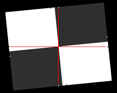
The use of guide marks for tilting the chart
|
The charts are printed straight and physically tilted because the edges print sharper that way. If they were printed at an angle, the printer dot pattern could result in some jaggedness. See Chart quality and distance in Imatest instructions part 1 for a detailed analysis. A 5.71 degree angle (tan-1(0.1)) is an offset of one part in 10. If you don't want to print your own chart, you can use the IMA/ISO 12233 target (available from Sine Patterns; expensive).
Assemble the prints into a target to be photographed.
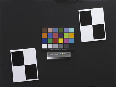 |
I mount the printed charts on a 32x40 inch sheet of 1/2 inch thick black foam board. 1/2 inch foam board stays flatter than standard 1/4 or 3/8 inch board. Black board results in less flare light than white board. (Flare light is light that bounces between lens elements and off the inside of the lens barrel, reducing image contrast)
Consider including charts for Imatest modules Colorcheck or Q-13 Stepchart. The Kodak Q-14 is more suitable than the Q-13 (shown on the left) because it is larger.
|
I use Velcro to attach the Colorchecker and Q-13 charts to the foam board so they can be easily removed. With Velcro, the surface of the Colorchecker is about 1/4 inch (6 mm) in front of the board. There is no need to remove the inexpensive printed charts, so I mount them on sheets of 1/4 inch foam board using 3M Photo Mount Spray Adhesive (or similar).
An image of a horizontal or vertical edge on an LCD monitor (desktop or laptop) can also be used as a target. The camera should be tilted with respect to the monitor. The image dark gray and white rather than black and white to minimize clipping. This page contains a description and an image.
Photograph the target.
|
Framing
I placed the the
upper right test chart near the center of the image and the lower
left test chart near the corner. The Colorchecker image is suitable for
analysis, but the the Q-13 is smaller than optimum. The dominant light
was from a skylight. The light was not as even as I would have
liked. |
|
Lighting
The chart below summarizes lighting considerations. The goal is even, glare-free illumination. Lighting angles around 30 degrees are ideal. Al least two lights (one on each side) is recommended; four is better. Beware of lights behind the camera, which can cause glare. Check before you expose.
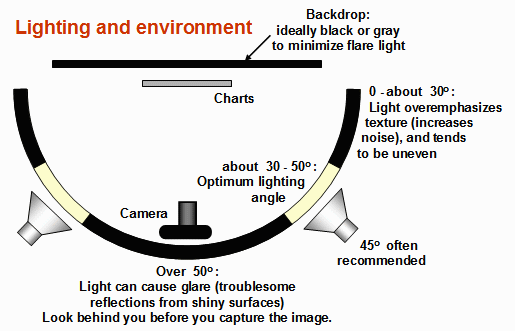
Distance
Using a letter-sized (8.5x11 inch) chart printed on Permium Luster paper on the Epson 2200 (a high quality pigment-based inkhet photo printer), the MTF of the 6.3 megapixel Canon EOS-10D showed no change if the image field was at least 22 inches (56 cm) wide-- twice the length of the chart. Performance falls off slowly for smaller widths. Choose a camera-to-target distance that gives at least this image field width. The actual distance depends on the sensor size and the focal length of the lens.
Cameras with more pixels, and hence higher potential resolution,
should
should have a larger image field width. Some gudelines for the minimum
field width are,
| Image field
width (in inches) > 8.8 * sqrt(megapixels)
( > means "greater than.")
Image field
width (in
cm) > 22
* sqrt(megapixels)
-- or --
The distance
to the target
should be at least 40X the focal length of the lens for digital SLRs.
(25X
is the absolute minimun; 40X leaves some margin.) For compact digital
cameras,
which have much smaller sensors, the distance should be at least 100X
the
focal length: the field of view is about the same as an SLR with
comparable
pixel count. The recommended distance is described in geeky detail in Chart
quality and distance. |
| The
camera-to-target
distance is not critical as long as it is greater than a reasonable
minimum. |
More on distance can be found in SFR Instructions Part 1.
|
Exposure
|
Proper exposure is important
for accurate Imatest SFR results.
Neither the black nor the white regions of the chart should clip--
have substantial areas that reach pixel levels 0 or 255. The best way
to
ensure proper exposure is to use the histogram in your digital camera.
Blacks (the peaks on the left) should be above the minimum and whites
(the
peak(s) on the right) should be below the maximum.
|
|
The histogram, taken from the Canon File Viewer Utility, indicates excellent exposure.
| Tips
on photographing the chart |
| Distance
doesn't matter
as long as the target far enough from the camera so sharpness is
limited
by the camera and lens, not
by the target. For a target printed on the Epson 2200 printer, a
distance
that gives at least a 24 inch (horizontal) field of view seems to be
sufficient. |
| The target
should be evenly
lit and free of glare. |
| White
balance should be
approximately neutral. |
| Use a
sturdy tripod and
a cable release. If possible, use the mirror lock. You can use Imatest
SFR to find the difference made by a good tripod or mirror lock-- to
sharpen
your technique, literally ( pun intended ). |
| Be sure to
expose the image
so detail is maintained in both light and dark areas. Neither should be
blocked (clipped). Use your camera's histogram. If more than 0.5% of
the
pixels are at levels 0 or 255, Imatest SFR will assume that clipping
has
taken place and issue a warning message. This has no effect on the
calculations--
it's just a warning that accuracy may be compromised. |
| Be sure
the camera is correctly
focused on the chart. |
| Place
slanted-edge images
near the corners of the field as well as near the center. |
| You may
find it instructive
to photograph the slanted edge target along with a target from Lens
testing, but there's no need to do so. |
|
Save the image as a RAW file or maximum quality JPEG. If you are
using
a RAW converter, convert to JPEG (maximum quality), TIFF (without LZW
compression,
which isn't supported), or PNG. If you are using film, develop and
scan
it. The file name should be descriptive and should indicate the
parameters
you are testing. Use dashes and underscores ( - and _ ), but avoid
spaces
(which work with Imatest, but can canse trouble in DOS command
lines
and web pages.) An example would be Canon_EOS10D_70-200f4L_100mm_f8.jpg.
Run Imatest SFR
These instructions are excerpted from Using Imatest SFR, Part 2 .
Imatest is opened by double-clicking the Imatest icon  on the Desktop, the Windows Start menu, or the Imatest directory (usually C:\Program files\Imatest). A fter several seconds, the Imatest main window opens. Then click on SFR: New File on the upper left. The SFR: Current file button is grayed out (inoperative) for the first run because no file has yet been read. It can be used in succeeding runs to save time when analyzing different regions, though multiple ROI (region of interest) runs are more efficient.
Select the image file
When you click SFR: New file, the window on the right appears, requesting the image file name. The folder saved from the previous run appears in the Look in: box on the top. You are free to change it. Double-click (or click and press Open ) to read the file name. Large files can take several seconds to load. Imatest remembers if you change the folder (for each module, individually). |
 |
Select the ROI (Region of Interest)
If the image has the same pixel dimensions as the last image in the previous run, a dialog box asks you if you want to repeat the same ROIs (regions of interest) as the previous image.
If you answer No or if the image has a different size, the image shown on the right is displayed with the instructions, Select ROI by clicking and dragging, or clicking outside image. Click on one corner of the intended region, drag the mouse to the other corner, then release the mouse button. Click outside the image to select the entire image. If the selected area is too small, too large, or inappropriate, you'll be asked to repeat the selection. If it is seems OK, a red outline will appear around the selection, an enlarged image of the selection will be displayed, and you'll be asked, Is the selected region OK? (below). You have five choices.
|
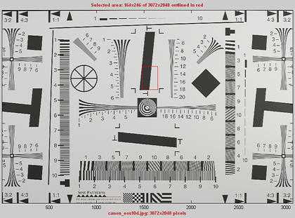
|
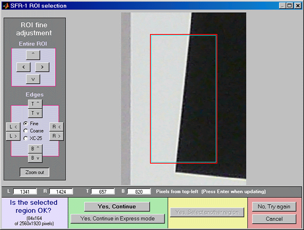 |
| Yes, Continue |
The selected ROI is correct; no more ROIs are to be selected. Continue with SFR calculations in normal mode: You will be asked for additional input data, etc. |
| Yes, Continue in Express mode |
The selected ROI is correct; no more ROIs are to be selected. Continue with SFR calculations in Express mode: You will not be asked for additional input data or for Save options. Saved or default settings will be used. |
| Yes, select another region |
The selected ROI is correct. Select another ROI. For multiple ROIs additional Figures will display performance as a function of distance from the image center. |
| No, try again |
The selected ROI is not correct. Try again. |
| Cancel |
Cancel the SFR run. Return to the Imatest main window. |
|
Cropping recommendations
Length should be between 80 and 500 pixels. Little is gained for length over 300 pixels. Width should be at least 60 pixels.
My typical crops are between around 120x80 and 240x140 pixels.
Widths for light and dark zones (shown on the right) should be at least 20 pixels. 30 is preferred. Little is gained for zone widths over 80 pixels. |
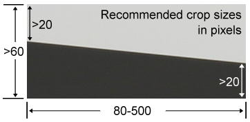 |
Additional SFR input
After you select the Region(s) of Interest (ROI(s)) the Imatest SFR input data window appears (unless Express mode has been selected). All input fields are optional. Most of the time you can simply click OK (the box on the lower right) to continue. The input data window is described fully in SFR instructions, Part 2. Here are a few highlights.
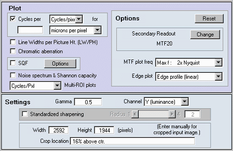 Plot controls which results are plotted. Plot settings are saved between runs. The boxes to the right of "Cycles per" control the x-axis display. You can choose between Cycles per pixel (the default), Cycles per inch, or Cycles per mm. If you choose Cycles per inch or mm, you must enter a number for the pixel size— either in pixels per inch, pixels per mm, or microns per pixel. An example is shown below for a plot in Cycles per mm for the Canon EOS-10D, which has a pixel spacing of 7.4 microns. If you omit this, the x-axis will be displayed in Cycles per pixel.
- Gamma is the exponent of the curve that relates scene luminance to pixel level. It is explained briefly in the glossary and in detail here. It defaults to 0.5, which is typical of digital cameras, but it is affected by camera (or RAW converter) contrast settings. Gamma is reliably 0.5 when RAW files are entered into Imatest (to be converted with dcraw). Gamma is used to convert pixel levels back to the linear scale required to calculate sharpness. A 10% error in gamma results in a 2.5% error in MTF50. If you have doubts about the value of gamma, I recommend running Colorcheck or Q-13 stepchart.
- Standardized sharpening radius controls the radius of the sharpening used to compensate for different amounts of sharpening in different digital cameras. Generally, the standardized sharpening results are not recommended for lens tests, though they can give a useful indication of what to expect after sharpening. The default value of 2 (pixels) is a typical sharpening radius for compact digital cameras, which have tiny pixels. The sharpening radius is sometimes smaller for digital SLRs, which have larger pixels, and can be different for different RAW converters. For more detail, see What is standardized sharpening, and why is it needed for comparing cameras?
When entries are complete, click OK. A Calculating... box appears to let you know that calculations are proceeding. Results appear in individual windows called figures (Matlab's standard method of displaying plots). Figures can be examined, resized, maximized, and closed at will. Their contents are described in MTF (Sharpness) plot, Chromatic Aberration, Noise, and Shannon Capacity plot, and Multiple ROI (Region of Interest) plot.
Two precautions when working with figures
Too many open Figures
Figures can proliferate if you do a number of runs, especially SFR runs with multiple regions, and system performance suffers if too many Figures are open. You will need to manage them. Figures can be closed individually by clicking X on the upper right of the Figure or by any of the usual Windows techniques. You can close them all by clicking Close figures in the Imatest main window. |
Clicking on Fgures during calculations
can confuse Matlab. Plots can appear on the wrong figure (usually distorted) or disappear altogether. Wait until all calculations are complete— until the Save or Imatest main window appears— before clicking on any Figures. |
Save the results
At the completion of the SFR calculations the Save results? dialog box appears (unless Express mode has been selected). It allows you to choose which results to save and where to save them. The default is subdirectory Results of the data file directory. You can change to another existing directory, but new results directories must first be created outside of Imatest using a utility such as Windows Explorer. (This is a limitation of this version of Matlab.)
When multiple ROIs are selected, the Save results? dialog box appears only after the first set of calculations. The remaining calculations use the same Save settings. Save results? is omitted entirely in an Express run for repeated images.
The first three check boxes are for the figures. The last three are for Excel .CSV results. You can examine the output figures before you check or uncheck the boxes. These selections are saved between runs. Details of the output files can be found here. |
 |
Repeated runs
If you have already run SFR and you click on either of the Run SFR buttons, and the new (or repeated) file has the same pixel dimensions as the previous file, an image that includes the selected ROIs appears on the left of the screen and you'll be asked, "Do you want the same ROIs as the previous image?" A portion of the previous image and the ROI repeat box, which contains the four answers, are shown in the image on the right.
|
|
The meaning of the answers is self-evident except for "Yes, Express mode."This button is the same as "Yes," except that the Input dialog box and the two Save dialog boxes (for individual Figures and for the multiple ROI figures at the end) are omitted. Default settings or settings saved from previous runs are used. The clipping warning boxes are suppressed. This speeds up repeated runs; for example, it's very handy when you are testing a lens at several apertures (f/2.8, f/4, f/5.6, etc.).
Interpret the results
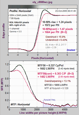 The most important of the Imatest SFR figures, shown on the right, contains the average edge profile on top and MTF (spatial frequency response) on the bottom. (Input-related data on the right of the figure is omitted here.)
Although the edge response in the upper figure is relevant to sharpness, the MTF curve in the lower figure is the preferred measurement because
- MTF, and especially MTF50, the spatial frequency where contrast drops to half its low frequency level, is a reliable indicator of perceived image sharpness, and
- System MTF response is the product of the MTF of individual components. No such simple formula is available for edge responses.
Although MTF50 is a reliable measurement of perceived image sharpness, other numbers can also be used for evaluating lenses.
For example, you could use MTF30 (which results in a higher spatial frequency), or MTF at a fixed spatial frequency (as is done in manufacturer's data sheets, which typically give contrast (MTF) at 10, 20, and 40 (or 10 and 30 line pairs/mm). If you do this you may want to scale the x-axis to cycles (i.e., line pairs) per mm instead of the default cycles/pixel.
Remember, in evaluating lenses, use the results without standardized sharpening (the black curves and text). Results with standardized sharpening do, however, have some interest: they indicate what can be achieved after sharpening. But they tend to "flatten" differences between lenses.
To learn more about sharpness measurements, see Sharpness: What is it and how is it measured?, SFR Tour, and SFR Results: MTF (Sharpness) plot.
Chromatic Aberration is an important aspect of lens performance. CA is best measured on tangential edges near the borders of the image. The best measure of CA is the percentage of the distance from the image center. Interpretation: under 0.04; insignificant. 0.04-0.08: minor; 0.08-0.15: moderate; over 0.15: serious.
For more information, see Chromatic Aberration and SFR Results: Chromatic Aberration ... plot. |
 |
Checklist
License holders are encouraged to publish test results in printed publications, websites, and discussion forums, provided they include links to www.imatest.com. The use of the Imatest Logo is encouraged. However you may not use Imatest for advertising or product promotion without explicit permission from Imatest LLC. Contact us if you have questions.
Imatest LLC assumes no legal liability for the contents of published reviews. If you plan to publish test results, you should take care to use good technique. Considerations include,
| Sturdy camera support |
Use a sturdy tripod, cable release, and, if possible, mirror-lock. |
| Target mounting |
If you are working outdoors, be sure the target doesn't shake in the wind. |
| Target distance |
Be sure you're far enough fro the target so the printed edge quality doesn't affect the measurements. Target distance considerations are given here. |
| Focus |
Be sure the camera is focused accurately on the target. Note whether you used manual or automatic focus. |
| Target alignment |
Make sure the corners, as well as the center, are in focus. |
| Raw conversion and settings |
The choice of RAW converter (in or out of the camera) and settings, particularly Sharpening, can make a huge difference. Contrast and White balance are also important. Settings that affect contrast and transfer curve can also have a strong effect. If possible a "Linear" setting (meaning a straight gamma curve with no additional tonal response adjustments) should be used.
|
Gamma
|
SFR sharpness results are moderately sensitive to the Gamma setting: A 10% gamma error changes MTF50 by 2.5%. For best results gamma should be measured by running Colorcheck or Q-13 Stepchart. Ideally a Q-14 target (similar to the Q-13, but larger) should be mounted close to the slanted edge images. |
| Cleanliness and filters |
Lens surfaces should be clean. You should note whether you have a protective (UV or Skylight) filter. It can make a difference— more likely reduced contrast than reduced sharpness. With Imatest you can find out. |
| File formats |
Use RAW or the highest JPEG quality. Never use less than the maximum resolution or JPEG quality unless you are specifically testing the effects of these settings. |
| Lens settings |
Lens performance is a strong function of the aperture (f-stop) and focal length (for zooms). Be sure to record these settings (easy because they're saved with the EXIF data) and include them in your writeup. The optimum (sharpest) aperture is of particular interest. Lens performance is also somewhat affected by the distance to the target. |
| White balance |
Should be close as possible to neutral, particularly in Colorcheck. |
This may seem like a lot of fuss, but the technique you develop in testing cameras and lenses will spill over to your daily photography. Alfred Stieglitz tested film and developers extensively when he discovered photography as a student in Berlin. Ansel Adams performed extensive tests in the development of his zone system. Although nobody would claim that testing is responsible for their unique vision, it certainly contributed to the skill they used to transform that vision into prints of transcendent beauty.
Installation
and getting started
Install Imatest
If you haven't dowloaded Imatest, go to the Imatest
download page before proceding. If you plan to install Imatest
on a computer that will not be conected to the Internet during
installation (or if you are behind a corporate firewall), download
the Matlab runtime library,
Imatest-lib.exe
(8.5 MB), to the same folder as the Imatest installer file. If Imatest-lib.exe is not in this folder during installation, the installer attempts to download
it from the Internet.
If
you have a personal firewall, be sure to disable it before you install
Imatest for the first time. You may re-enable it as soon as the installation
is complete. This should not be necessary on subsequent installations.
Open Windows Explorer and double-click on the Imatest installer file, Imatest-version.exe.
(Version is the version number. The Change Log contains the update history.) The version is displayed in the welcome window. Follow the instructions
in the installation wizard (mostly clicking
Next
>). The Imatest installation requires approximately 34 MB
(mostly the Matlab libraries).
If you encounter difficulties go to the Troubleshooting
page.
Imatest can be run by clicking the Imatest icon  on the Desktop, the Start menu, or in the Imatest installation folder (C:\Program
files\Imatest in English language installations). Instructions for running Imatest
are located in Imatest instructions.
Links to instructions for individual Imatest
modules are located in the Imatest Documentation
page.
When you first run Imatest,
it will be in evaluation mode, which allows up to 20 runs of individual
modules. Evaluation mode has all the capabilities of the registered
version except for two.
- It does not save results files.
- There is a watermark in the background of the plots.
Purchase
Imatest
You may purchase Imatestat any time from Regsoft.com's secure site. The introductory price is $59
US. You will be entitled to updates for one year from the date of purchase.
You can also click on the Purchase
button in the Imatest main window.
After you purchase Imatest you'll receive two e-mails. (1) An immediate confirmation
of your purchase. (2) A confirmation that your credit card has been accepted.
This may take a few minutes. You may register Imatest as soon as you receive
this e-mail; it contains the password you need to register. These e-mails
are cluttered with text from Regsoft. The password is near the middle.
Register
imatest
After you've purchased Imatest you'll need to register it by clicking on the Register button in the Imatest main window. It's a good idea to check the Imatest
download page to be sure you have the latest version.
If
you have a personal firewall, be sure to disable it before you register.
You may re-enable it as soon as registration is complete. If you can't disable it, follow the instructions below, then continue with Offline registration.
Fill in the the Register Imatest
window: Enter your name, company (if applicable), e-mail, and the password
you received in the second Regsoft e-mail, then click on Register.
If you forgot your password, click on Recover
password. This opens a website, www.imatest.com/lostpassword,
that enables you to recover your lost password via e-mail.

If your computer is connected to the internet, you will receive a confirmation of your registration, and the full version of Imatest will be activated immediately.
Offline registration
If your computer is offline, or if you are unable to connect because
of a firewall that can't be disabled, the following box appears.

Click on Manual activation. The box below appears with instructions
for manual registration. Steps 2-4 can be performed on any computer connected
to the internet.

On www.imatest.com/activate, fill in all the fields as shown below, then click Make Activation Code . Don't leave any fields blank— always enter something. Your code will be e-mailed to you. Enter it into the Activation key: field, above.

Reminder: For offline installation, the Matlab runtime library,
Imatest-lib.exe (8.5 MB), must be downloaded to the same folder as the Imatest installer file.
Files
When the installation
is complete the Imatest folder should contain the following folders and
files.
The default installation
folder for Imatest is C:\Program files\Imatest.
(It may differ in non-English
installations.)
.
| samples (folder) |
Contains several image files
with sample data for testing the three Imatest modules. Includes
several
cropped JPEG files for testing SFR, indicated by _sfr in their names.
Canon_EOS10d_ColorCheck_lt_small.jpg — for testing Colorcheck.
Canon_EOS10D_Q13_ISO400_small.jpg — for testing Q-13.
Edge_chart.png and Edge_chart_low.png — the printable SFR edge images.The latter
(low contrast) is recommended.
|
| images (folder) |
Contains several image files
used by Imatest. |
| bin (folder) |
Contains the .fig files
used in the graphic user interface (GUI), as well as Matlab library files.
Includes FigureMenuBar.fig and FigureToolBar.fig: library files missing
from Imatest-lib.exe. |
| toolbox (folder) |
Subdirectories contain Matlab
library files (mostly DLLs). |
 Imatest
 |
(full name Imatest.lnk)
The standard icon for running Imatest. Runs start.bat, which sets the path
then runs imatest.exe. Copied to Windows Start Menu and Desktop. |
 Diagnoistics
 |
(full name Diagnostics.lnk)
Runs Imatest in diagnostic mode. Doesn't close when Imatest terminates.
This allows error messages to be viewed. Runs diagnostics.bat, which sets
the path then runs imatest.exe. |
| jhead.exe |
DOS application for reading
EXIF data (digital camera information). |
| dcraw.exe |
Dave Coffin's dcraw RAW conversion program. |
| imatest.exe |
Imatest executable program. |
start.bat
imadiag.bat |
Batch files that set the
Windows Path and run Imatest.exe. Diagnostics.bat is used for diagnostic
mode: the DOS window remains open if Imatest terminates with an error. |
Using Imatest
Running Imatest
Imatest can be run from the Start menu ( Start > All Programs > Imatest >  Imatest ) or by double-clicking the Imatest icon
 on the Desktop or in the Imatest folder. This opens the Imatest main window, shown below.
Imatest modules are run by clicking on one of the buttons on the upper left. (More will be added as Imatest evolves.) Instructions for the individual modules are on their own pages: SFR, Colorcheck, and Q-13 Stepchart .
The following steps are common to all Imatest modules.
-
Open the image file. A dialog box requests the name of the input image file. Imatest supports
TIFF (24 or 48-bit; without LZW compression), JPEG, PNG (24 or 28-bit), BMP, HDF, PCX, XWD, and PPM (24 or 28-bit) file
formats. It also supports RAW files for a large variety of digital cameras, using Dave Coffin's dcraw. New cameras are typically added to dcraw within one to three months of their introduction. The dcraw page has the latest list of cameras.
-
Crop, if desired. When the input image is opened, the entire image is displayed. The message, Select the ROI by clicking & dragging, or click outside the image, appears above
the image.
Select the crop area (Region of Interest) by clicking on an intended corner and dragging the
mouse to another corner. If you don't want to crop the image— if you want
to use the entire original image, click outside the image. Note: the Zoom feature of Matlab Figures
 does not work during region selection. Imatest mistakely assumes you are trying to select the entire image. To enlarge the image (to view the crop area more clearly), maximize it by clicking on the square next to the upper right corner of the Window.
- Verify your selection, which appears in a separate figure unless you selected the entire image by clicking outside of it. Imatest also
checks the crop for validity. If it is invalid, the input image reappears
with an error message.
-
Enter additional input data. A dialog box requests the Title (which defaults to the file name)
and other data, depending on the module. All additional data isoptional; you only need to pay attention if you wish to change the defaults. Click OK to continue or Cancel to terminate
the run.
-
Run the program by clicking OK. The results are presented in individual Figures.
- Save results? A dialog box asks if you would like to save the results. Checkboxes in
the dialog box enable you to select the Figures to be saved. You may examine
the results before deciding which, if any, to save. (This box is omitted in the evaluation version.)
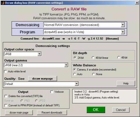
About RAW files
RAW files are the unprocessed output of digital image sensors. For Bayer sensors, each RAW pixel represents a single color in RGRGRG, GBGBGB, ... sequence. To be converted into usable, standard file formats (TIFF, JPEG, etc.), raw files must be processed by a RAW converter (de-mosaicing) program. RAW converters perform additional functions: they apply the gamma curve, often an additional tonal response curve; they also reduce noise and sharpen the image. Thse operations can interfere with several of Imatest's measurements.
The only way you can be sure an image file faithfully resembles the RAW file— that it has a pure gamma curve, no sharpening, and no noise reduction— is to read a RAW file into Imatest using Dave Coffin's dcraw, which converts it to PPM format. If you select any of the standard RAW formats (CRW, NEF, etc.) the dialog box on the right appears. It allows you to choose among several RAW conversion options.
For 24-bit conversion the default gamma is 0.5. For 48-bit conversion the Gamma box is grayed out and gamma is fixed at 1 (not an ideal value). Fuji Super CCD files may be rotated 45 degrees.
Dcraw converts RAW files into PPM files— an obscure format not supported by all image editors. If check the box to delete the converted (PPM) file, you may save the image in one of three standard formats: TIFF (uncompressed), PNG (lossless compression; takes longer), or JPEG (lossy compression; maximum quality; 24-bit only).
A list of supported cameras appears on the dcraw site. New cameras are typically added within one to three months of their introduction. |
Other controls
Exit closes all figures and terminates Imatest.
Close figures closes all figures. You may close figures individually by the usual Windows methods — clicking
the X in the upper right or
right-clicking on the figure icon on the Taskbar and selecting Close.
Expand hi res figs applies only to high resolution screens (1600x1200 pixels and above). When this box is checked (by default), images are enlarged so they don't look tiny on the screen. Unchecking the box turns this feature off. Images are smaller but better suited for website presentation. The setting is saved between runs.
Small / Normal / Large fonts alters the font size in output
figures and GUI windows. The default is Normal.
The setting is saved between runs. This address problems with tiny fonts in high resolution
screens (1600x1200 pixels and above)
or larger than expected fonts which appear when the video card DPI setting
is Large size (120 DPI) instead of Normal. The video card setting can be accessed by
right-clicking on the Windows background, then clicking Properties, Settings,
Advanced, General (tab). Large fonts are displayed if DPI is set to Large size (120
DPI). 96 DPI is normal. You have to reboot Windows
before new settings take effect.
Saved settings: Imatest saves a number of settings, including Font size, folders for opening and
saving images (for all modules), plot selection (for SFR), and save figure
selection (for SFR and Colorcheck). To restore these settings to their
original defaults, click the File menu
(at the top of the Imatest window), then click Reset defaults,
Yes. The settings are stored in Imatest.ini.
Figures
Imatest results are displayed in individual windows called figures.
A typical figure— the result of running SFR for the Canon EOS-10D— is
shown below.
|
Figures
may be resized, minimized, maximized, or closed using standard Windows
operations. In addition, several Windows and Matlab-specific operation
can be found in the toolbar at the top of the image.

The first four icons
in the toolbar are standard Windows icons: New file, Open, Save, and Print.
Open and Save refer to Matlab .fig figures, which can only be opened from
the Matlab program or a Matlab figure window. Imatest allows you to save figures as PNG files— an excellent format with lossless
compression.
Of the remaining three icons, the most useful is Zoom
in:  .
Clicking on it highlights it and enables you to zoom in on regions of the
plots. You can click and drag to create a zoom rectangle or you can click
on any point to zoom in on that point. Double-clicking anywhere on the image
restores the magnification to its initial state .
Clicking on it highlights it and enables you to zoom in on regions of the
plots. You can click and drag to create a zoom rectangle or you can click
on any point to zoom in on that point. Double-clicking anywhere on the image
restores the magnification to its initial state
|

Imatest figure: You can resize it or zoom in on individual plots.
|
Two precautions when working with Figures
|
Too many open Figures
Figures can proliferate if you do a number of runs, especially SFR runs with multiple regions,and
system performance suffers if too many Figures are open. You will need to manage them. Figures
can be closed individually by clicking X on the upper right of the
Figure or by any of the usual Windows techniques. You can close them all
by clicking Close figures in the Imatest main window.
|
Clicking on Figures during calculations
Plots can appear on the wrong figure (usually distorted) or disappear altogether.
Wait until all calculations are complete— until the Save or Imatest main
window appears— before clicking on any Figures.
|
To see Figure resource use, open the Windows Task Manager. In Windows XP, click
Control-Alt-Del or right-click in the Taskbar, usually at the bottom of
the screen. Click on the Processes tab, then click CPU twice so the tasks
with the most CPU usage appear at the top. Imatest can be a real CPU hog when several Figures are open; CPU use appears to increase with the
square of the open Figures. On my dual 1 GHz Pentium Windows XP machine,
8 open Figures use 6% of the CPU; 16 open Figures use 33%. Over 20 would
seriously slow the computations.
Use of Imatest
The Imatest license allows an individual user to install and use the
software on (A) a maximum of three computers (for example, home, laptop,
and office) used exclusively by a single individual, or (B) a single workstation
used nonsimultaneously by multiple people, but
not both. It is not a concurrent use license.
License holders are encouraged to publish test results in printed publications,
websites, and discussion forums, provided they include links to www.imatest.com.
The use of the Imatest Logo is encouraged. However you may not use Imatest
for advertising or product promotion without explicit permission from
Imatest LLC. Contact us if you have questions.
Imatest LLC assumes no legal liability for the contents of published
reviews. If you plan to publish test results, you should take care to use
good technique. Considerations include,
| Sturdy camera support |
Use a sturdy tripod, cable
release, and, if possible, mirror-lock. |
| Target mounting |
If you are working outdoors,
be sure the target doesn't shake in the wind. |
| Target distance |
Be sure you're far enough
fro the target so the printed edge quality doesn't affect the measurements.
Target distance considerations are given
here. |
| Focus |
Be sure the camera is focused
accurately on the target. Note whether you used manual or automatic focus. |
| Target alignment |
Make sure the corners, as
well as the center, are in focus. |
| Raw conversion and settings |
The choice of RAW converter
(in or out of the camera) and settings, particularly Sharpening, can make a
huge difference. Contrast
and White balance are also important. Settings that affect contrast and
transfer curve can also have a strong effect. If possible a "Linear"
setting (meaning a straight gamma curve with no additional tonal
response adjustments) should be used.
|
Gamma
|
SFR
sharpness results are moderately sensitive to the Gamma setting: A 10%
gamma error changes MTF50 by 2.5%. For best results gamma should be
measured by running Colorcheck or Q-13 Stepchart. Ideally a Q-14 target (similar to the Q-13, but larger) should be mounted close to the slanted edge images.
|
| Cleanliness and filters |
Lens surfaces should be
clean. You should note whether you have a protective (UV or Skylight) filter.
It can make a difference— more likely reduced contrast than reduced sharpness.
With Imatest you can find out. |
| File formats |
Use RAW or the highest JPEG
quality. Never use less than the maximum resolution or JPEG
quality unless you are specifically testing the effects of these settings. |
| Lens settings |
Lens performance is a strong
function of the aperture (f-stop) and focal length (for zooms). Be
sure to record these settings (easy because they're saved with the EXIF
data) and include them in your writeup. The optimum (sharpest) aperture
is of particular interest. Lens performance is also somewhat affected by
the distance to the target. |
| White balance |
Should be close as possible
to neutral, particularly in Colorcheck. |
This
may seem like a lot of fuss, but the technique you develop in
testing cameras and lenses will spill over to your daily photography. Alfred
Stieglitz tested film and developers extensively when he discovered photography
as a student in Berlin. Ansel Adams performed extensive tests in the development
of his zone system. Although nobody would claim that testing is responsible
for their unique vision, it certainly contributed to the skill they used
to transform that vision into prints of transcendent beauty.
Using SFR Part 1
Setting up and photographing the target
The
slanted-edge test image
Imatest SFR
measures the
spatial frequency response, also known as the Modulation
Transfer Function (MTF), of digital cameras and digitized film
images.

ISO 12233 test chart
with Imatest SFR cropping
indicated by the red rectangle.
It uses a simple slanted-edge (black-to-white) target described in Sharpness:
What is it and how is it measured? Although it doesn't provide the as strong a visual indication of MTF as the test described in Lens testing, it provides a far more accurate quantitative measurement.
Imatest SFR also measures Chromatic aberration, noise and Shannon
information capacity— a useful but unfamiliar indicator of image
quality.
Imatest SFR uses a standardized sharpening algorithm to compensate for the different amounts of sharpening in different cameras, allowing them to be fairly compared.
The algorithms for calculating MTF/SFR were adapted from a Matlab program, sfrmat, written by Peter Burns to implement the ISO 12233 standard. The original Matlab code is available on the I3A download page on ISO 12233 Slant Edge Analysis Tool sfrmat 2.0. You can write Peter at  .
.
A horizontal slanted-edge for measuring vertical MTF
performance is
shown below; a vertical slanted-edge for measuring horizontal MTF
performance
is shown on the right. These edges were cropped from an image of the
PIMA/ISO
12233 test chart taken by the Canon EOS-10D digital SLR, shown above. A crop area is indicated by a red rectangle. |

|

|
Printing,
assembling, and photographing the target
Although Imatest SFR
works splendidly
with the
IMA/ISO 12233
target (available from Sine
Patterns; expensive),
you can run it with any clean, sharp, straight black-to-white or dark
gray-to-white
edge. The solid areas need to be smooth and uniform: white on one side
and black or dark gray on the other. Since Imatest
does not yet sell a printed chart (it's planned), the quickest way to
obtain
a chart is to download a file and print it on a high quality inkjet
printer.
Download a test chart.
You
can download a printable test chart by right-clicking on one of the
thumbnails
below. (These charts are included in the samples folder of the Imatest
installation.) The chart on the left, which has pixel levels 47 and
255,
has a contrast ratio of (255/47)2.2 = 41 when printed
at gamma = 2.2 (the normal setting). This is close to the minimum
recommended
by the ISO 12233 standard. The chart on the right, which has pixel
levels
0 and 255, prints with the maximum possible contrast ratio for the
printer/paper
combination, typically between 80:1 and 100:1. This may result in
clipping
near the edges in some cameras. For this reason the reduced contrast
chart
on the left is recommended.
A printable vector-graphics version of the ISO 12233chart is available courtesy of Stephen H. Westin of the Cornell University Computer Graphics Department. If you use it, you should print it as large as possible so edge sharpness is not limited by the printer itself. (There may be some jaggedness in the slanted edges; not a problem with the recommended target.)
Print the charts
|
with a high quality inkjet
photo printer on glossy, semigloss, or luster paper. I recommend
printing
at least two copies: one for measuring center sharpness and one for
edge
sharpness. The printed image size should be 8x10
inches (20.3x25.4 cm) or smaller—
its size is not critical. Be sure the edges look clean and sharp to
your
eyes; examine them with a good magnifier or loupe. Chart quality is
described
in geeky detail in Chart quality and distance,
below.
The charts are intended to be tilted approximately 5.7 degrees
(anywhere
between 4 and 7 degrees is OK) when they are photographed. It is tilted
5.7 degrees when the tick marks, located near the edges, are vertically
or horizontally aligned with the center. This is illustrated by the red
horizontal and vertical lines on the right.
|

The use of guide marks for tilting the chart
|
The charts are printed straight and physically tilted because the
edges
print sharper that way. If they were printed at an angle, the printer
dot
pattern would result in a slight jaggedness. A 5.71 degree angle ( = tan-1(1/10))
is an offset of one part in 10.
Assemble the charts into a target
to be photographed.
 |
If you are using other Imatest
modules, such as Colorcheck or Q-13,
you may want to combine charts.
I used a 32x40 inch sheet of 1/2
inch thick black foam board for the assemblage. The 1/2 inch foam board
stays flatter than standard 1/4 or 3/8 inch board. Black board results
in less flare light than white board. (Flare light is light that
bounces
between lens elements and off the inside of the lens barrel, reducing
image
contrast) |
I use Velcro to attach the Colorchecker and Q-13 charts to the foam
board. That makes them easy to remove. With Velcro, the surface of the
Colorchecker is about 1/4 inch (6 mm) in front of the board.
There is no need to remove the inexpensive printed charts, so I
mount
them on sheets of 1/4 inch foam board using 3M Photo Mount Spray
Adhesive
(anything similar will do), then I mount the foam board using RTV
silicone
seal, which can be removed without much damage.
An image
of a horizontal or vertical edge on an LCD monitor (desktop or
laptop)
can also be used as a target. The camera should be tilted with
respect
to the monitor. (Thanks to Scott
Kirkpatrick for the suggestion.)
 |
To minimize artifacts (Moire, etc.) the camera must be
far enough from
the monitor so the sensor pixel "frequency" (1/(2*pixel
spacing) at the image sensor) is at least 30% above the Nyquist
frequency
of the LCD screen. A good rule of thumb is that the LCD screen image
should
take up no more than 1/3 to 1/4 the image width (1/9 to 1/16 the area),
as shown on the right.
My inexpensive Toshiba laptop, shown on the right,
displays 1024 pixels
horizontally. The Canon EOS-10D has 3072 horizontal pixels. In this
case,
the laptop image should take up no more than 1/4 the image width. |
Click here to view a web page
with a suitable
LCD test image (dark gray and white rather than black and white to
minimize clipping).
|
Photograph the target.
|
I placed the the
upper right test chart near the center of the image and the lower
left test chart near the corner. The Colorchecker image is suitable for
analysis, but the the Q-13 is smaller than optimum. The dominant light
was from a skylight. The light was not as even as I would have
liked.
|
|
Lighting
The chart below summarizes lighting considerations. The goal is even, glare-free illumination. Lighting angles around 30 degrees are ideal. Al least two lights (one on each side) is recommended; four is better. Beware of lights behind the camera, which can cause glare. Check before you expose.

Distance
|
|
Using a letter-sized (8.5x11
inch) chart printed on Permium Luster paper on the Epson 2200 (a high
quality
pigment-based inkhet photo printer), I analyzed the MTF performance of
the 6.3 megapixel Canon EOS-10D. I found no change if the image field
was
at least 22 inches (56 cm) wide— twice the length of the chart.
Performance
falls off slowly for smaller widths. Choose a camera-to-target distance
that gives at least this image field width. The actual distance depends
on the sensor size and the focal length of the lens. The minimum image
field is illustrated on the right.
|
|
Cameras with more pixels, and hence higher potential resolution,
should
should have a larger image field width. Some gudelines for the minimum
field width are,
Image field
width (in inches) > 8.8 * sqrt(megapixels)
( > means "greater than.")
Image field
width (in
cm) > 22
* sqrt(megapixels)
— or —
There should
be no more
than 140 sensor pixels per inch of target or 55 sensor pixels per
centimeter
of the target.
— or —
The distance
to the target
should be at least 40X the focal length of the lens for digital SLRs.
(25X
is the absolute minimun; 40X leaves some margin.) For compact digital
cameras,
which have much smaller sensors, the distance should be at least 100X
the
focal length: the field of view is about the same as an SLR with
comparable
pixel count. The recommended distance is described in geeky detail in Chart
quality and distance, below. |
| The
camera-to-target
distance is not critical as long as it is greater than a reasonable
minimum. |
|
Exposure
|
|
Proper exposure is important
for accurate Imatest SFR
results.
Neither the black nor the white regions of the chart should clip—
have substantial areas that reach pixel levels 0 or 255. The best way
to
ensure proper exposure is to use the histogram in your digital camera.
Blacks (the peaks on the left) should be above the minimum and whites
(the
peak(s) on the right) should be below the maximum.
|
|
The above image (taken from the Canon File Viewer Utility) is close
to a perfect exposure.
| Tips
on photographing the chart |
| Distance
doesn't matter
as long as the target far enough from the camera so sharpness is
limited
by the camera and lens, not
by the target. For a target printed on the Epson 2200 printer, a
distance
that gives at least a 24 inch (horizontal) field of view seems to be
sufficient. |
| The target
should be evenly
lit and free of glare. |
| White
balance should be
approximately neutral. |
| Use a
sturdy tripod and
a cable release. If possible, use the mirror lock. You can use Imatest
SFR to find the difference made by a good tripod or mirror lock— to
sharpen
your technique, literally ( pun intended ). |
| Be sure to
expose the image
so detail is maintained in both light and dark areas. Neither should be
blocked (clipped). Use your camera's histogram. If more than 0.5% of
the
pixels are at levels 0 or 255, Imatest SFR will assume that clipping
has
taken place and issue a warning message. This has no effect on the
calculations—
it's just a warning that accuracy may be compromised. |
| Be sure
the camera is correctly
focused on the chart. |
| Place
slanted-edge images
near the corners of the field as well as near the center. |
| You may
find it instructive
to photograph the slanted edge target along with a target from Lens
testing, but there's no need to do so. |
|
Save the image as a RAW file or maximum quality JPEG. If you are
using
a RAW converter, convert to JPEG (maximum quality), TIFF (without LZW
compression,
which is not supported), or PNG. If you are using film, develop and
scan
it. The file name should be descriptive and should indicate the
parameters
you are testing. Use dashes and underscores ( - and _ ), but avoid
spaces.
(Spaces work with Imatest, but they can be troublesome in DOS command
lines
and web pages.) An example would be Canon_EOS10D_70-200f4L_100mm_f8_ctr.jpg.
You are now ready to run
Imatest
SFR.
| Chart
quality and distance |
Three printed charts were scanned with the Epson 3200
flatbed scanner
at 1200 dpi— a much higher scan density than normal for reflective
documents
(300 or 400 dpi). At a typical monitor resolution of 96 dpi, the images
are enlarged 12.5x. The charts were tilted around 5.7 degrees (a 1.1
inch offset on an
11 inch letter-sized print) for analysis with Imatest SFR.

Epson 2200
Premium Glossy 1440 dpi
High contrast
|
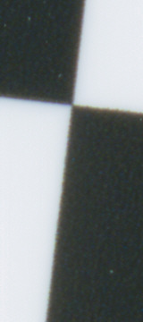
Epson 2200
Premium Glossy
1440 dpi
Reduced contrast
|
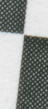
HP LaserJet 5L
bond paper
Reduced contrast
|
The high contrast chart appears to be the
sharpest. The reduced contrast
chart is still very good: its dot pattern (always a concern) is not a
problem.
The laser print is clearly unsuitable.
Results of running Imatest
SFR on the high contrast printed chart are shown below. The SFR input
dialog
box was set to display cycles/millimeter for 1200 pixels/inch (scan
density).
The key result is MTF50 (50% contrast spatial frequency) = 5.15
cycles/millimeter
(131 cycles/inch). Results in LW/PH and with standardized sharpening
(indicated
by (corr.); dashed red lines) are not
applicable.
As expected, the reduced contrast chart, which
doesn't appear as sharp,
has a lower MTF50: 4.31 cycles/mm (109 cycles/inch). It would benefit
from
sharpening in the image editor.
The chart MTF50 affects the minimum recommended
camera-to-target distance.
For example, the Canon EOS-10D (and 300D) has a pixel spacing of 7.4
microns.
Its Nyquist frequency is 1000/(2*7.4) = 68
cycles/mm.
When the target is 40x the lens
focal
length, so the magnification at the sensor is approximately 1/40
(recommended
above), the MTF50 imaged on the sensor for the reduced contrast chart
is
4.31*40 = 172 cycles/mm, which is 2.5 times the Nyquist frequency. The
imaged target contrast is approximately 0.9 in the critical region
around
0.6*Nyquist (0.3 cycles/pixel). This is adequate, though a little more
distance) (e.g., 50x focal length)
wouldn't hurt. |
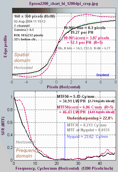
|
A print of Stephen H. Westin's printable vector-graphics version of the ISO 12233chart, made on the Epson 2200 at 1440 dpi on Premium Luster paper and scanned by the Epson 3200 at 1200 dpi, has been analyzed to compare slanted and straight edges. The comparison is of interest because Stephen's chart uses vector graphics, hence the slanted edge is as fine as the printer can make; it is not limited by image pixels. Straight and slanted edges where compared with the print scanned straight and tilted.
The straight edge is clearly smoother than the slanted edge, though the sharpness of the individual edges (horizontal scan lines) is about the same. This MTF results are surprizing: MTF50 for the slanted edge scanned straight is 4.13 cycles/mm, not very different from MTF50 for the straight edge scanned tilted, 4.24 cycles/mm. The difference is more pronounced at lower MTFs (higher spatial frequencies). MTF20 for the slanted edge scanned straight is 8.6 cycles/mm while MTF20 for the straight edge scanned tilted is 10.6 cycles/mm. I clearly perfer the straight edge, tilted. Although the numbers suggest it would make little difference, I recommend a 20% greater distance if the slanted edge is used. |
|
Imatest SFR LCD target
The test pattern below is dark gray and white rather than black and white because LCD screens
can have extremely high contrast-- 400:1 or more-- enough to cause clipping,
which reduces the accuracy of Imatest SFR measurements.
|
When you display this taget
on a LCD screen, be sure to maximize the browser window. To avoid Moire
fringing (interference between the LCD and camera sensor pixels) and chromatic
aberration from the R-G-B pixel pattern, the LCD screen image should take
up no more than 1/3 to 1/4 the width of the total image (1/9 to 1/16 the
area).
My inexpensive Toshiba laptop, shown on the right, displays 1024 pixels
horizontally. The Canon EOS-10D has 3072 horizontal pixels. In this case,
the laptop image should take up no more than 1/4 the image width.
|
|
Since the screen occupies only a small portion of the image area, be sure the camera is focused on the screen!
The first two zones are 1000
pixels high; the remaining zones are 600 pixels high. Scroll down to locate
the edge of choice.
The pattern contrast was reduced slightly on August
1, 2004.
Return to Imatest SFR instructions
Using SFR Part 2
Using Imatest SFR
Running
Imatest SFR
Imatest is opened by double-clicking the Imatest icon  on
on
- the Desktop,
- the Windows Start menu,
- or the Imatest directory (usually C:\Program files\Imatest).
After several seconds, the Imatest main window, shown below, opens. Then click on one of the SFR buttons on the upper left. The SFR: Current file button is grayed out (inoperative) for the first run because no file has yet been read. It can be used in succeeding runs to save time when analyzing different regions, though multiple ROI (region of interest) runs are more efficient.

Several cropped slanted-edge JPEG images are included in the images
subdirectory of the Imatest directory. Complete ISO12233 charts are not
included with Imatest because they are large (usually over 2 megabytes).
They can be downloaded from dpreview.com reviews, typically in the last page titled "Compared to...," and from Imaging-resource.com reviews, typically on the page labeled "sample images."
Selecting
the image file
|
When you click SFR: New file,
the window on the right appears, requesting the image file name. The folder
saved from the previous run appears in the Look
in: box on the top. You are free to change it. An image file
for the Canon EOS-10D is highlighted. Double-click (or click and press
Open )
to read the file name. Large files can take several seconds to load. Imatest
remembers if you change the folder (for each module, individually).
|
 |
Selecting
the ROI (Region of Interest)
If the image has the same pixel dimensions as the last image in the previous run, a dialog box shown below asks you if you want to repeat the same ROIs (regions of interest) as the previous image.
|
If you answer No or if the image has a different size, the image shown on the right (reduced) is displayed.
The instructions are, Select
ROI by clicking and dragging, or clicking outside image.
Click on one corner of the intended region, drag the
mouse to the other corner, then release the mouse button. Click outside
the image to select the entire image. If the selected area is under 2500
pixels, over 200,000 pixels, or appears to be inappropriate, you'll be
asked to repeat the selection. If it is seems OK, a red outline will appear
around the selection, an enlarged image of the selection will be displayed,
and you'll be asked, Is the selected region
OK? (below). You have five choices. |

|
Note: the Zoom feature of Matlab Figures  does not work here. Imatest mistakely assumes you are trying to select the entire image. To enlarge the image (to view the crop area more clearly), maximize it by clicking on the square next to the upper right corner of the Window.

|
| Yes, Continue |
The selected ROI is correct;
no more ROIs are to be selected. Continue with SFR calculations in normal
mode: You will be asked for additional input data, etc. |
| Yes, Continue in Express mode |
The selected ROI is correct;
no more ROIs are to be selected. Continue with SFR calculations in Express
mode: You will not be asked for additional input data or for Save options.
Saved or default settings will be used. |
| Yes, select another region |
The selected ROI is correct.
Select another ROI. For multiple ROIs additional Figures will display performance
as a function of distance from the image center. |
| No, try again |
The selected ROI is not
correct. Try again. |
| Cancel |
Cancel the SFR run. Return
to the Imatest main window. |
|
|
Cropping recommendations
Length should be between 80 and 500 pixels. Little is gained for length
over 300 pixels. Width should be at least 60 pixels.
My typical crops are between around 120x80
and 240x140 pixels.
Widths for light and dark zones (shown on the right) should be at least 20 pixels.
30 is preferred. Little is gained for zone widths over 80 pixels.
|
 |
Additional
SFR input
 The Imatest SFR data window, shown on the right, appears after the Region of
Interest (ROI) has been selected, unless Express mode has been chosen.
It appears only once during multiple ROI runs. Succeeding runs have the
same entries except for Crop location.
All input fields are optional. Most of the time you can simply click OK (the button on the lower right) to continue.
Title
defaults
to the input file name. You may leave it unchanged, replace
it, or add descriptive information— as
you please.
Plot
controls which results are plotted. Plot settings are saved between runs.
Only the Cycles per (pixel) and Chromatic Aberration plots are checked by default. The LW/PH plot
is unchecked (by default) because it is largely redundant.
The boxes to the right of "Cycles
per" control the x-axis display. You can choose between
Cycles
per pixel (the default), Cycles
per inch, or
Cycles
per mm. If you choose Cycles
per inch or mm,
you must enter a number for the pixel size— either in pixels
per inch,
pixels
per mm, or microns
per pixel. An example is shown below for a plot in Cycles
per mm for the Canon EOS-10D, which has a pixel spacing of
7.4 microns. If you omit this, the x-axis will be displayed in Cycles
per pixel.
If both Chromatic Aberration and Noise spectrum and Shannon capacity are checked, the two plots share the same figure: CA on top and Noise/Shannon capacity at the bottom. Noise spectrum and Shannon capacity is unchecked by default because there results are difficult for most users
to interpret.

Picture Width and Height defaults
to the width and height of the input image in pixels, assuming landscape format,
where height < width. If the input image
has been cropped, or if it doesn't represent the entire camera image, Picture
Height (and Width) should be entered manually.
Line Width per Picture Height (LW/PH) results are correct only if the
Picture Height represents the entire uncropped frame. For example, Picture
Height should be set to 2048 for the Canon EOS-10D and 1944 for the Canon
G5 (the cameras in the cropped sample files), etc.
| For
film and scanner users |
| More film/scanner users
than I expected are using Imatest. And film users prefer
results in Line Pairs per mm (LP/mm). You can select cycles (line pairs)
per inch or millimeter in the Plot
box. Scanned images tend to be cropped by the time they are entered into Imatest because complete images are
huge. (Try running the numbers for a 4,000 dpi scanner.) In this case, you
must manually enter the picture height in pixels to get LW/PH. The best way
is to use the equation, |
|
Picture height (pixels) = picture height (mm) * pixels/mm. |
| For example, a 4,000 dpi scanner has 4000/25.4
= 157.5 pixels/mm. For 35mm film, the picture height is 24 mm = 3780 pixels.
With medium format cameras, the picture height is somewhat smaller than
the nominal size. It is 41.5 mm for the 645 format and 56mm for the 6x6
and 6x7 (cm) formats. Picture Width is optional, but it's a good idea to enter it. It is calculated in the same way. |
|
Channel
is normally left at it's default value of Y for the luminance channel,
where Y = 0.3*R + 0.59*G + 0.11*B.
In rare instances the R, G, and B color channels might be of interest.
Gamma is
used to linearize the input data (explained below). It defaults to 0.5
= 1/2, which is typical of digital cameras, but is affected by camera (or RAW converter) contrast settings. It may
be quite different for scanned film images.
Since SFR sharpness measurements are moderately sensitive to the
Gamma setting (a 10% error in gamma results in a 2.5% error in MTF50), it's a good idea to run Colorcheck or Q-13 stepchart to determine the correct value of Gamma.
| Gamma |
Gamma is the exponent of the equation that relates image pixel
level to luminance. For a monitor or print,
Output luminance
= (pixel level)gamma
When the raw output of the image sensor,
which is linear, is converted to image file pixels with a standard color space,
the approximate inverse of the above operation is applied.
pixel level
= (RAW pixel level)gamma_camera ~= exposuregamma_camera
The total system gamma is gamma
* gamma_camera. Standard values of (output) gamma are 1.8 for color
spaces used in the Macintosh and 2.2 for color spaces used in Windows, such as
sRGB
(the default when color space is unspecified) and Adobe RGB (1998).
In
characteristic curves for film and paper, which use logarithmic scales (e.g.,
density (log10(absorbed light) vs. log10(exposure)),
gamma is the average slope (excluding the "toe" and "shoulder"
regions near the ends of the curve), i.e.,
gamma is contrast.
See Kodak's
definition in Sensitometric
and Image-Structure Data.
To obtain the correct MTF, Imatest must linearize the pixel levels; the camera's gamma must be removed.
That is the purpose of Gamma
in the SFR input dialog box, which defaults to 1/2,
typical of a wide range of digital cameras. It can, however, vary
considerably with camera and RAW converter settings, most notably
contrast.
Characteristic curves for the Canon EOS-10D with three RAW converter
settings are shown on the right. Gamma deviates considerably from 0.5.
Gamma = 0.679 could result in a 9% MTF50 error. For best accuracy I
recommend measuring
gamma using
Colorcheck or Q-13 Stepchart, which provides slightly more detailed results.
Confusion factor: Digital
cameras rarely apply an exact gamma curve: A "tone reproduction curve" (an
"S" curve) is frequently superposed on the gamma curve to extend dynamic range while maintaining visual contrast.
This reduces contrast in highlights and (sometimes)deep shadows while maintaining
it in middle tones. You can see it in curves 1 and 3, on the right. For
this reason, "Linear response" (where no S-curves is applied on top of
the gamma curve) is recommended for SFR measurements.
The transfer function may also be adaptive:
camera gamma may be higher for low contrast scenes than for
contrasty scenes. This can cause headaches with SFR measurements. But
it's not a bad idea generally; it's quite similar to the development
adjustments (N-1, N, N+1, etc.) in Ansel Adams' zone
system. For this reason it's not a bad idea to place a Q-13 or Q-14 chart near the slanted edges.
To learn more about gamma, read Tonal
quality and dynamic range in digital cameras and Monitor
calibration. |
In
characteristic curves, which use Log scales, gamma is defined as the
average slope of the transfer function, excluding the extreme
highlights and shadows.
The three curves below, produced by Q-13 Stepchart for the Canon EOS-10D, show how Gamma varies with RAW converter settings.
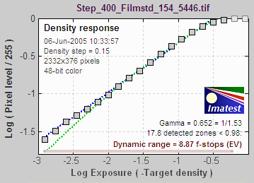 1. Capture One LE set to Film standard (the default). Gamma = 0.679.

2. Capture One LE set to Linear response. Gamma = 0.508. Recommended for SFR runs.
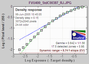
3. Canon FVU set to Standard contrast. Gamma = 0.642.
|
|
Standardized sharpening
radius controls the radius of the sharpening used to
compensate for different amounts of sharpening in different digital cameras.
Its default value of 2 (pixels) is a typical sharpening radius for compact
digital cameras, which have tiny pixels. The sharpening radius is sometimes
smaller for digital SLRs, which have larger pixels, and can be different
for different RAW converters. Although a value of 2 is recommended
for comparing cameras, you may occasionally want to experiment with the
sharpening radius. Results with standardized sharpening should not be used
for comparing different lenses on the same camera. For more detail, see
What
is standardized sharpening, and why is it needed for comparing cameras?
Crop location
is the position of the center of the selected ROI (Region of interest),
expressed as the percentage the distance from the image center to the corner.
The orientation of the ROI with respect to the image center is included.
It is blank if the input image has not been cropped. Crop location can
be entered manually. This is only recommended when that image has been
cropped outside of Imatest SFR.
Additional parameters
(all optional) for Excel .CSV output EXIF data
is entered, if available. These settings are optional but useful when several
tests are run for different lenses, focal lengths, apertures, or other
settings.
Save settings
If checked, most parameters are retained for additional runs. This is useful
when the same camera and lens is tested at a number of apertures and focal
lengths. Saved settings are overridden by EXIF data, if it is present.
Some settings can change between runs: Description is always reset to the
input file name and Picture Height and Width are calculated from the input
file. Location is calculated for each Region of Interest (ROI).
When entries are complete, click OK.
A Calculating...
box appears to let you know that calculations are proceeding. Results appear
in individual windows called Figures (Matlab's standard method
of displaying plots). Figures can be examined, resized, maximized, and
closed at will. Their contents are described in the pages on Imatest
SFR results: MTF (Sharpness) plot, Chromatic Aberration, Noise, and Shannon Capacity plot, and Multiple ROI (Region of Interest) plot.
Two precautions
when working with figures
Too
many open Figures
Figures can proliferate
if you do a number of runs, especially SFR runs with multiple regions,
and
system performance suffers if too many
Figures are open. You will need to manage them. Figures
can be closed individually by clicking X on the upper right of the
Figure or by any of the usual Windows techniques. You can close them all
by clicking Close figures in the Imatest main window. |
Clicking
on Figures during calculations
can confuse Matlab. Plots
can appear on the wrong figure (usually distorted) or disappear altogether.
Wait until all calculations are complete— until the Save or Imatest main
window appears— before clicking on any Figures. |
Saving
the results
|
At the completion of the SFR calculations the Save
results? dialog box appears, unless Express mode has
been selected. It allows you to choose which results to save and where
to save them. The default is subdirectory
Results
of the data file directory. You can change to another existing directory,
but new results directories must first be created outside of Imatest using
a utility such as Windows Explorer. (This is a limitation of this version
of Matlab.)
When multiple ROIs are selected, the Save
results? dialog box appears only after the first set
of calculations. The remaining calculations use the same Save settings.
Save
results? is omitted entirely in an Express
run for repeated images.
The first three check boxes are for the figures. The last three are
for Excel .CSV results. You can examine the output figures before you check
or uncheck the boxes. After you click on Yes
or No, the Imatest
main window reappears. These selections are saved between runs. |
 |
Result file
names— The roots of the file names are
the same as the image file name. The channel (Y, R, G, or B) is included
in the file name. If a Region of Interest has been selected from a complete
digital camera image, information about the location of the ROI is included
in the file name following the channel. For example, if the center of the
ROI is above-right of the image, 20% of the distance from the center to
the corner, the characters AR20 are included in the file name.
Output files
for canon_eos10d.jpg (Y-channel)
(in
subdirectory Results)
| Figures
(.PNG image files) |
| canon_eos10d_YA17_cpp.png |
Plot with x-axis in cycles/pixel (c/p), Y-channel,17% of the way to
the corner above the center of the uncropped image. |
| canon_eos10d_YA17_lwph.png |
Plot with x-axis in Line Widths per Picture Height (LW/PH). |
| canon_eos10d_YA17_ca.png |
Plot of Chromatic Aberration, with noise statistics and Shannon information
capacity. |
| Excel
.CSV (ASCII text files) |
| SFR_cypx.csv |
(Database file for appending results: name does not change). Displays
10-90% rise in pixels and MTF in cycles/pixel (C/P). Described below. |
| SFR_LWPH.csv |
(Database file for appending results: name does not change). Displays
10-90% rise in number/Picture Height (/PH) and MTF in Line Widths per Picture
Height (LW/PH). Described below. |
| canon_eos10d_YA17_MTF.csv |
Excel .CSV file of MTF results for this run. The first row has the
headers: cy/pxl, LW/PH, MTF, MTF(corr). The remaining lines contain the
data. Can easily be plotted or combined with data from other files. |
The third file is identical to the Imatest
Figure (below), except that the background is white instead of gray.

These results are explained in Sharpness: What is it and how is it measured?
Repeated
runs
|
If you have already run SFR and you click on either of the Run
SFR buttons, and the new (or repeated) file has the same pixel
dimensions as the previous file, an image that includes the selected ROIs
appears on the left of the screen and you'll be asked, "Do
you want the same ROIs as the previous image?" A portion
of the previous image and the ROI repeat box, which contains the four answers,
are shown in the image on the right.
|
|
The meaning of the answers is self-evident except for "Yes,
Express mode."This button is the same as "Yes,"
except that the Input dialog box and the two Save dialog boxes (for individual
Figures and for the multiple ROI figures at the end) are omitted. Default
settings or settings saved from previous runs are used. The clipping warning
boxes are suppressed. This speeds up repeated runs; for example, it's very
handy when you are testing a lens at several apertures (f/2.8, f/4, f/5.6,
etc.).
Excel
.CSV (Comma Separated Values) output
Imatest SFR creates or updates output files for use
with Microsoft Excel. The files are in CSV (comma-separated values) format,
and are written to the results directory. CSV files are ASCII text files
that look pretty ugly when viewed in a text editor:
File
,Date/time
,PH,Ch,H/V,10-90U,10-90C,Over-,Over-,MTF50U,MTF50C,MTF,Camera,Lens,FL,f-stop,Loc,Misc.
,,,,,/PH,/PH,shoot%,sharp%,LW/PH,LW/PH,Nyq,,,(mm),,,settings
canon_eos10d_sfr.jpg,2004-03-19
22:21:34, 2048,Y,H, 1422, 1447, 19.5, -0.7, 1334, 1340,0.154,,,,,
canon_g5_sfr.jpg,2004-03-19
22:24:30, 1955,Y,H, 1973, 1301, 48.0, 21.3, 1488, 1359,0.268,Canon G5,—,14,5.6,ctr,
sigma_sd9_sfr.jpg,2004-03-19
22:27:55, 1504,Y,H, 1432, 1676, 2.4, -7.7, 1479, 1479,0.494,,,,,
sigma_sd10_sfr.jpg,2004-03-19
22:28:32, 1504,Y,H, 1563, 1628, 11.9, -2.0, 1586, 1587,0.554,,,,, |
But they look pretty decent when entered into
Excel.

CSV files can be edited with any of the usual
text editors: Notepad, Write (WordPad), etc, but it makes far more sense
to edit them in Excel, where columns as well as rows can be moved and/or
deleted. Some fields are truncated in the above display, and Date/time
is displayed as a sequence of pound signs (#####...).
The format can be changed by dragging the boundaries between cells on
the header row (A, B, C, ...) and by selecting the first two rows and setting
the text to Bold. This makes the output look better. The modified
file can be saved with formatting as an Excel Worksheet (XLS) file. This,
of course, is just the beginning.

It's easy to customize the Excel spreadsheet to your liking.
For example, suppose you want to make a concise chart. You can delete Date/time
(Row B; useful when you're testing but not so interesting later) and Channel
(all Y = luminance). You can add a blank line under the title, then you
can select the data (rows A4 through J7 in the image below) and sort on
any value you choose. Corrected MTF50 (column I) has been sorted in descending
order. Modified worksheets should be saved in XLS format, which maintains
formatting.

There are no limits. But I've said enough. ( I'm not an
Excel expert! )
Database
files
Two .CSV files are used as a database for storing data from SFR runs.
If possible, data from the current run is appended to these files. A third
file for storing MTF data is described below.
-
SFR_cypx.csv displays 10-90% rise in
pixels and MTF in cycles/pixel (C/P).
-
SFR_lwph.csv displays 10-90% rise in
number/Picture Height (/PH) and MTF in Line Widths per Picture Height (LW/PH).
When SFR is run, it looks for the two files in the same folder as the slanted-edge
input image. If it doesn't find them, it creates them, writes the header
lines, then writes a line of data for the run. If it finds them, it appends
data for the run to the files. You can rapidly build a spreadsheet by doing
repeated runs from files in the same folder. The following table contains
the entries. Camera and the entries
that follow are all optional. With the exception of Loc,
which is calculated when the ROI is manually selected, they are only added
if you answer y
to the question, Additional
data for Excel file?, and enter them manually.
| File |
File name. Should be concise
and descriptive. |
| Date/time |
Date and time in sortable
format. Displays differently in Excel. |
| PH |
Picture Height (in SFR_lwph.csv
only). |
| Ch |
Channel. Y (luminance) [default],
R, G, or B. |
| H/V |
Horizontal or Vertical measurements.
(A vertical chart
gives you horizontal rise and MTF, etc.) |
| 10-90U |
10-90% rise distance, uncorrected. |
| 10-90C |
10-90% rise distance, corrected
with standard sharpening. |
| Overshoot% |
Overshoot of the edge. |
| Oversharp% |
Oversharpening: the amount
of sharpening relative to the standard sharpening.
If negative, the image is
undersharpened. |
| MTF50U |
MTF50 (frequency where MTF
= 50%), uncorrected. |
| MTF50C |
MTF50 (frequency where MTF
= 50%), corrected with standard sharpening. |
| MTF Nyq |
MTF at Nyquist frequency.
Indicates likelihood of aliasing problems. |
| Camera |
Camera name. This entry
and those that follow are manually-entered and optional. |
| Lens |
Lens name. Only for DSLRs
with interchangeable lenses. |
| FL (mm) |
Focal length in mm. |
| f-stop |
Aperture |
| Loc |
Location of image (center,
edge, corner, etc.) |
| Misc. settings |
Anything else: RAW converter,
Sharpening setting, etc. |
Tips
-
To build a spreadsheet of results, put the slanted-edge image files in
the same folder. File names should be concise and descriptive. If you've
run SFR from image files in different folders, there will be multiple versions
of the CSV files. They can be easily combined with a text editor on in
Excel.
-
Neither SFR_cypx.csv nor SFR_lwph.csv should be open in Excel when you
run SFR. If either is open, an error message will appear instructing you
to close them.
Other .CSV
files
|
Imatest writes a file that contains .CSV data for MTF. The file name
is [root name]_MTF.csv. The format is shown on the right. The columns
are
-
Spatial frequency in the units chosen for the "Cycles per" plot (cycles/pixel,
cycles/mm, or cycles/in),
-
Spatial frequency in LW/PH,
-
MTF, and
-
MTF (corrected, i.e., with standardized sharpening).
|
|
cy/pxl, LW/PH,    MTF, MTF(corr)
0.0000,  0.00, 1.0000,    1.0000
0.0059, 28.97, 0.9934,    0.9931
0.0118, 57.94, 0.9931,    0.9922
|
|
SFR Results: MTF (Sharpness) plot
Edge response and Spatial Frequency Response (MTF)
Imatest SFR displays Edge profiles and SFR plots in one or two Figures. The first displays spatial frequency in Cycles per Pixel (C/P) or Cycles per distance (inches or mm). The second displays spatial frequency in Line widths per picture height (LW/PH; shown below). It is only plotted if the corresponding checkbox in the Imatest SFR input dialog box has been checked. (It is unchecked by default.) Note that one cycle (or line pair) is equivalent to two line widths.
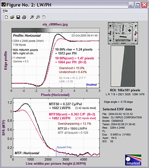
The most important results below are shown in Bold. The most important is MTF50, without and with Standardized sharpening. Its relationship with print quality is discussed in Interpretation of MTF50.
Upper left: Edge profile plot |
|
| Black line (bold) |
Edge profile for the luminance (Y) channel, where Y = 0.3*R + 0.59*G + 0.11*B. Original (without standardized sharpening). |
Red line
(dashed, bold) |
Edge profile for the luminance (Y) channel with standardized sharpening. Radius R used for setting standardized sharpening is displayed. Defaults to 2, but may set manually; may be larger for unusually broad transitions (poor MTF response). |
R, G, and B
dashed lines (thin) |
Individual edge profiles for R, G, and B channels. Shown more prominently in the Chromatic Aberration plot, below. Barely visible in this illustration because this camera has very little chromatic aberration. |
Left column text
(input settings) |
| Title, including measurement orientation. (A vertical edge is used for a horizontal profile.) |
| Image height (H) or Width x Height (WxH) in pixels |
| Total megapixels |
| Channel. Defaults to Y (luminance). R, G, or B are also available. |
| Gamma is an estimate of camera gamma used to linearize the image. Defaults to 0.5. |
| Region of interest (ROI) size in pixels |
| ROI location in percentage of distance from center to corner. |
|
Right column text
(results) |
| 10-90% rise distance (original; uncorrected) in pixels and rises per picture height (PH). |
| 10-90% rise distance (with standardized sharpening; corrected) in pixels and rises per PH. Radius R used for setting standardized sharpening is displayed. Defaults to 2, but may set manually; may be larger for unusually broad transitions (poor MTF response). Includes the equivalent "ideal megapixels" in brackets [...]. |
| Overshoot and undershoot. Percentage of step amplutide. Shown if appropriate. |
| Average pixel levels in dark and light areas, and light/dark ratio. Clipping can occur if they are too close to 0 or 255. Also gives the ratio between the light and dark areas: an indication of the contrast of the image. |
|
| Right: Input data |
| |
Top right image
Thumbnail of the entire image, showing the location of the selected region of interest (ROI) in red. |
| |
Middle right image
The selected region of interrest (ROI), shown with the correct aspect ratio, but not necessarily the exact size. |
| |
Lower right text
Selected EXIF data: Data recorded by the digital camera. Only for JPEG files. May include ISO speed, aperture, and other details. Thanks to Matthias Wandel for jhead.exe. |
|
|
 |
Lower left:
Spatial frequency response (MTF) plot
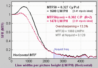 |
|
| Black line (bold) |
Spatial Frequency Response (MTF) for the luminance (Y) channel. Unprocessed. |
Red line
(dashed,bold) |
Spatial Frequency Response (MTF) for the luminance (Y) channel with Standardized sharpening. |
Right column text
(results) |
| MTF50
(50% contrast spatial frequency) for the original uncorrected image
in cycles/pixel and line widths per picture height (LW/PH). Its relationship to print quality is discussed in Interpretation of MTF50. |
| MTF50
(with standardized sharpening; corrected) in cycles/pixel and
LW/PH. Radius R used for setting standardized sharpening is displayed.
Defaults to 2 (larger for unusually broad transitions (poor
MTF response)). It may be adjusted in the input dialog box. |
| Equivalent "ideal megapixels" in brackets [...]: a number
based on the concept that the "ideal" pixel would have an MTF of 1 up to
the Nyquist frequency (0.5 C/P), and 0 above, and hence, MTF50 = 0.5 C/P.
The number of "ideal pixels" that would yield the identical sharpness is, |
|
4 * MTF50(C/P horizontal) * horizontal pixels * MTF50(C/P vertical) * vertical
pixels |
| The number displayed assumes
that MTF50 is the same in horizontal and vertical directions— usually
a pretty good assumption, especially with standardized sharpening. But
there are exceptions, such as the Nikon D70. You should not expect the
"ideal megapixel" count to equal the total megapixel count of the camera.
In the real world, performance is excellent if it is half the actual megapixels. |
|
| Oversharpening or undersharpening.The amount the camera is over- or undersharpened with respect to standardized
sharpening. |
| MTF30 (30% contrast spatial
frequency) for the original uncorrected image. |
MTF at the Nyquist
frequency.An indicator of the effectiveness of the anti-aliasing filter and
likelihood
of aliasing effects such as Moire patterns. Aliasing effects are
insignificent
under 0.1. They can become serious over 0.3. There is a tradeoff: the
more
effective the anti-aliasing, the worse the sharpness. Foveon sensors
(used in the Sigma SD9 and SD10) are more tolerant of aliasing than Bayer sensors, which are used in most digital cameras.
|
| Nyquist frequency: Half
the sampling rate = 1/(2*pixel
spacing). Always 0.5 cycles/pixel. Indicated by the vertical blue line. |
|
SFR Results: Chromatic Aberration, Noise, and Shannon capacity plot
Chromatic Aberration, noise, and Shannon capacity
The camera chosen for the plot below has significant Chromatic Aberration. The Noise spectrum and
Shannon capacity plots, shown below beneath Chromatic Aberration,
are plotted only if the Noise Spectrum and Shannon capacity (in CA plot) checkbox in the Imatest SFR input dialog box has been checked. It is unchecked by default.
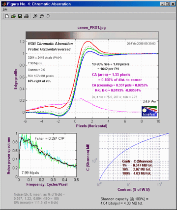
| Upper plot: Chromatic Aberration |
 |
| More about this plot can be found in the page on Chromatic Aberration. Much of this plot is grayed out if the ROI is too close to the center for reliable CA measurements (less than 30% of the distance to the corner). |
Red, Green, and Blue
lines (bold) |
Edge profiles for the R, G, and B channels (original, uncorrected). (Standardized sharpening is not used for chromatic aberration.) |
| Black line (dashed) |
Edge profile for the luminance (Y) channel. |
| Dashed magenta line (bold) |
The difference between the highest and lowest channel levels. (All channels are normalized to go from 0 to 1.) The visible chromatic aberration is proportional to the area under this curve. |
| Left column text |
Input settings: Plot title, profile orientation (Horizontal profile corresponds to a vertical edge, etc.), image dimensions (WxH), total megapixels, gamma, ROI size, ROI location. |
Right column text
(results) |
| 10-90% rise distance (original; uncorrected) in pixels and rises per picture height (PH). |
| CA (Area): Chromatic aberration area in pixels. An indicator of the severity of CA. The area between the channels with the highest and lowest levels. In units of pixels because the x-axis is in pixels and the y-axis is normalized to 1. Explained in the page on Chromatic aberration. Meaning (now obsolete): Under 0.5; insignificant. 0.5-1: minor; 1-1.5: moderate; 1.5 and over: serious. |
| Chromatic aberration based on the edge centers (where the edges cross 0.5). This is generally smaller than CA (equiv.) and also less indicative of the visibility of the CA. |
| CA: Chromatic aberration as a percentage of the distance to image center. A better indicator than pixels (above). Equal to 100 * (CA in pixels) / (distance from center in pixels), corrected for the edge angle. Relatively independent of the ROI location because CA tends to be proportional to the distance from the image center. It is also independent of the number of pixels in the sensor. Explained in the page on Chromatic aberration. Meaning: Under 0.04; insignificant. 0.04-0.08: minor; 0.08-0.15: moderate; over 0.15: serious. |
| Average pixel levels in the dark and light areas. Clipping can occur if they are too close to 0 or 255. |
|
| Lower part of figure: Noise and Shannon information capacity plots |
 |
| for for the selected channel, normally luminance (Y) |
Noise spectrum plot
(left side) |
The noise spectrum plot
is somewhat experimental; its meaning will become clearer. Bayer interpolation causes a rolloff in the noise spectrum; noise reduction causes additional rolloff, which may be unusually rapid for strong noise reduction.
Lower frequency noise components tend to be more visible. The spiky light cyan
and green curves represent two different
directions.
The thick black line is the smoothed average of the two. The red line is a third order polynomial fit to the noise. |
Shannon capacity plot
(right sde) |
Shannon capacity C
as a function of signal S (closely related to image Contrast), where S is expressed as the percentage of the difference between the white
and black regions of the target (Sstd ). A Contrast of 100% represents a fairly contrasty image, 10% represents
a low contrast image, and 1% represents a smooth area like skies. These numbers
are only meaningful for comparing digital cameras. They should be used with caution because signal processing, especially noise reduction, has a strong effect on Shannon Capacity. There is
a table of results in the page on Shannon
information capacity. |
| Text at bottom |
| Noise in the dark and light
areas, and the mean of the two. Measured after the input data has been
linearized (corrected for the gamma encoding). Expressed as a fraction
of the difference between the average levels of the light and dark areas (Sstd ).
This difference is the standard signal, S, used in the calculation of Shannon
information capacity. The noise measurements in Q-13 Stepchart and Colorcheck are more reliable and useful. |
| Signal-to-noise ratio S/N
for the mean of the light and dark areas. This is the inverse of the noise
for the mean of the light and dark areas, above. Used in the calculation
of Shannon capacity. |
| Shannon
information capacity of the camera for signal S =
Sstd,
measured in bits per pixel and megabytes total. This is an approximate
calculation that provides an estimate of overall image quality for moderately
contrasty images, as affected by sharpness and noise. |
|
SFR Results: Multiple ROI (Region of Interest) plot
Multiple regions of interest
Imatest SFR allows you to
select several regions of interest (ROIs). When more than one is selected,
two composite Figures are produced. Each figure contains two plots: MTF50 (upper left) and 10-90% rise distance (lower left) as a function of distance from the center of the image, scaled as the percentage of distance from center to corner (0 = center; 1 = corner). The two figures differ in scaling: the first is relative to pixels; the second is relative to image height.. These figures show performance (MTF50 and rise distances without
and with standardized sharpening) in Cycles/Pixel (or Cycles/mm or Cycles/inch)
and Line Widths/Picture Height. The first Figure also plots Chromatic
Aberration.
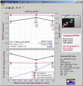
The most important results below are shown in Bold. Illustrations are for the first figure (Cycles per pixel in this case).
| Upper left: MTF50 (Half-contrast frequency)
|
|
| This plot shows MTF50 (the half-contrast spatial frequency) as a function of distance from the center of the image, scaled as the percentage from center to corner (0 = center; 100 = corner). There are two vertical (y) axes. The primary axis is on the left; the secondary axis (italicized) is on the right. These alternate for the two plots. In this plot, the primary axis is in Cycles/pixel for MTF50 and Pixels for 10-90% rise distance. It can also be in Cycles/mm or Cycles/inch if specified in the SFR data window. |
Black line (bold) |
MTF50 (half-contrast spatial frequency) for the luminance (Y) channel. Unprocessed. This is the number to use for measuring lens sharpness. |
Red line
(bold, dashed) |
MTF50 for the luminance (Y) channel with Standardized sharpening. This is the number to use when making general comparisons of different cameras with different degrees of sharpening. |
Symbols and numbers
below data points,
top to bottom |
| Orientation: Location of region relative to image center. A = Above, B = Below, L = Left, R = Right. |
| MTF50, Uncorrected and with Standardized sharpening, in units corresponding to the primary vertical (y) axis scale on the left. The vertical order is determined by the order of the data points, i.e., if the Uncorrected MTF50 is higher, its value is on top. |
| MTF50, Uncorrected and with Standardized sharpening, in units corresponding to the secondary vertical (y) axis scale on the right. These numbers are italicized. The vertical order is determined by the order of the data points, i.e., if the Uncorrected MTF50 is higher, its value is on top. |
|
| Right column: Crop, Results summary, and EXIF data |
Top right image
Thumbnail of the entire image, showing the locations of the selected regions of interest (ROI) in red.
|
Middle right box:
Weighted MTF50
Results summary
|
Summary of key results of multiple ROI runs:
Weighted mean values for MTF50, in cycles per ... and LW/PH units, without and with standardized sharpening. The MTF value at the middle of each (sorted) line segment is weighted according to the length of the line segment and the distance from the center: the center is weighted twice as strongly as the corner. These weights are used to calculate a weighted mean. This algorithm prevents closely spaced points from being given excessive weight. |
Lower right text
Selected EXIF data: Data recorded by the digital camera. Only for JPEG files. May include ISO speed, aperture, and other details. Thanks to Matthias Wandel for jhead.exe. |
|
 |
|
Lower left: 10-90% Edge
rise distance
|
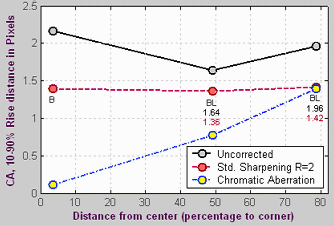 The Legend at the lower right of the 10-90% Rise distance plot sometimes covers data points. It can be moved by clicking and dragging it with a mouse.
 |
|
Black line
(bold)
|
The 10-90% rise distance,
uncorrected (without Standardized sharpening). |
|
Red
line
(bold,
dashed)
|
The 10-90% rise distance, with Standardized sharpening. |
|
.Blue
line
(bold,
dashed)
with
yellow
circles.
|
Chromatic
aberration (Area-based) in pixels. An indicator of the severity
of CA. The area between the channels with the highest and lowest levels.
In units of pixels because the x-axis is in pixels and the y-axis is normalized
to 1. Explained in detail in the page on
Chromatic
aberration. Meaning: Under 0.5; insignificant. 0.5-1: minor;
1-1.5: moderate; 1.5 and over: serious. |
Using Q-13 Stepchart
Introducing Q-13 Stepchart
Q-13 Stepchart analyzes the tonal response,
noise,
and dynamic range of digital cameras and scanners using
Q-13 Stepchart produces more detailed results than Colorcheck.
The Kodak Q-13 Gray Scale is an 8 inch long
chart
consisting of 20 zones, labeled 0-19, which have optical
densities from 0.05 to 1.95 in steps of 0.1 (reflectances from
0.891
to 0.011). The chart is printed on a
(semigloss)
surface. The Jessops chart, from the UK, is similar to the Q-13, except that it has only 18 zones.
| This
image of the Q-13 Gray Scale was photographed
slightly
out of focus to minimize noise. |
 |
The Q-13 has finer steps and a higher maximum density than the
GretagMacbeth
ColorChecker (Dmax = 1.95 vs. 1.5), mostly because of its glossier
surface. It considerably less
expensive. Kodak also makes a 14 inch long Q-14, which is identical
with
the Q-13 except for its length. It can be used in
exactly
the same way. It's well suited for photographing next to slanted-edge
SFR
test targets.
Iliah Borg has analyzed the Q-13 Gray Scale. He says, "I'm pretty sure it's screen-printed, most likely with automotive
enamel. The spectral response is flat from 420 to 730nm,
similar to titanium dioxide mixed with carbon in different
proportions to achieve different reflectivities. The layer is
pretty thick, to isolate from the substrate."
Q-13 Stepchart also analyzes transmission (i.e., film) charts, which
have higher maximum densities than reflective charts, making them
valuable
for measuring the dynamic range of digital cameras and scanners, as
discussed
below, in the section on Dynamic range.
Photographing
the chart and running Q-13 Stepchart
- Photograph the chart. Be sure the light is even. As little as
possible
should come from behind the camera— it can cause glare and flatten
image
tones. An angle of incidence of about 30 degrees is ideal for lighting.
The light should not emphasize the texture of the chart, which would
cause
an error in the noise measurement. At least two lamps are recommended.
If possible, the surroundings of the Step chart should be dark gray or
black to minimize flare light. Tips on lighting can be found here.
- The chart may be photographed slightly
out of focus to minimize noise measurement errors due to texture in the
patches. I emphasize slightly—
the boundaries between the patches must remain distinct.
- The distance at which the target is photographed is not critical.
The
noise
analysis will work well if the total cropped chart length is at least
1000
pixels (about 50 pixels per zone), about 1/3 the width of the image in
a 6 megapixel digital SLR. Increasing the size improves the accuracy of
the noise measurement.
- Save the image as a RAW file or maximum quality JPEG, then load
it on
your
computer. If you are using a RAW converter, convert to JPEG (maximum
quality),
TIFF (without LZW compression, which is not supported), or PNG. If you
are using film, develop and scan it.
- Click on the Q-13 Stepchart
button in the Imatest main window.
- Open the input file using the dialog box. Imatest remembers the
directory
name of the last input file opened (for each module, individually).
- Crop the image to minimize edge effects. A typical crop is shown
below.
Click outside the image for no crop. The orientation does not
need
to be correct; Imatest will rotate the image to the correct orientation.

- Make any needed changes to the Q-13 Stepchart input dialog box. A
reflective
target with density steps of 0.10 (the Kodak Q13/Q14) is selected by
default.
If you are using a transmission target, be sure to choose the correct
target
type. (See Dynamic range, below.) Click OK
to continue.

Output
The example was photographed with the Canon EOS-10D at ISO 100 and
converted
from RAW format using Capture One with default settings (no curves
applied).
The results include tonal response and noise. Colorcheck
produces a similar result, but with less tonal detail. Two figures are
produced.

First
Figure
The upper plot shows the average density
of the
Q-13 grayscale patches (black curve) and first and second order
density fits (dashed blue and green
curves). The horizontal axis is the distance along the target. A
portion of the patches themselves are shown just above the plot. The
equations
for the density fits are given in the Algorithm section, below. The
second
order fit closely matches the patches. The light cyan spikes are the
differentiated
and smoothed steps used to find the boundaries between zones.
The lower plot shows the RMS noise for
each patch:
R, G, B, and Y (luminance), expressed as the percentage of the range of
pixel levels corresponding to a target density range of 1.5: the same
as
the white - black patches on the ColorChecker.
The high levels of Red and Blue noise in zones 1-6 may be due to
imperfections
in the target. These imperfections are completely swamped by the noise
at ISO 1600, below. Noise is largest in the dark areas because of gamma
distortion: In the conversion from the sensor's linear output to the
color
space (sRGB, here) intended for viewing at gamma = 2.2, the dark areas
are amplified more than the light areas, hence their noise appears to
be
greater.
|
The second Figure contains the
most important of the results: the response curve (displayed on a log
scale, similar to film response curves), the noise expressed in two
different ways (most meaningful as a fraction of an f-stop or EV), and the
dynamic range (for
transmission step charts). The horizontal
axis for the three plots on the left is Log Exposure, which equals
(minus) the nominal target
density
(0.05 - 1.95 for the Q-13).
The upper left plot shows the density response (gray squares), as well as the first and second order fits (dashed blue and green lines). It resembles a traditional film density response curve. Dynamic range is grayed out because the reflective Q-13 target has too small a dynamic range to measure a camera's total dynamic range. See Dynamic range, below.
|
The upper right box contains dynamic range results: total dynamic range and range for several quality levels, based on luminance (Y) noise. It is shown in gray when a reflective target is selected. |
Second figure
|
 |
The middle left plot
shows noise in f-stops (or EV) ,
i.e., noise scaled to (divided by) the
difference in pixel levels between f-stops, which decreases as
brightness decreases. The darkest levels have the highest noise. This
measurement corresponds to the workings of the eye and has
important consequences for the calculation of practical dynamic range.
The vertical axis is logarithmic to display low noise levels clearly.
Dynamic range information is displayed when the range for a specific
quality level (defined by maximum noise) is within the range of the
plot..
|
EXIF data is shown in the
middle right region.
|
The bottom left plot
shows the noise scaled to the difference in pixel levels between the
maximum density level and the patch corresponding to a density of 1.5—
the same density range as the GretagMacbeth Colorchecker. It may be less visually
meaningful then the middle plot.
|
The lower right plot
shows the noise
spectrum. Digital
camera images with excessive noise reduction will have an unusually
rapid
falloff of the noise spectrum. |
Here are the results for ISO 1600. Tonal response is similar to ISO
100,
but the noise is greatly increased— enough to swamp out any
imperfections
in the target. The noise is highly visible. It wouldn't be suitable for
portraits and other high quality work, but it would be acceptable when
a grainy "Tri-X" or "available light" look is desired. Neat
image
can do an excellent job of reducing it. The middle-left plot displays
dynamic range for several quality levels, specified by the maximum
noise within the range. The dynamic range for low quality (L; blue) has a maximum noise of 1 f-stop; the dynamic range for high quality (H; yellow) has a maximum noise of 0.1 f-stop.
Saving
the results
|
When the Q-13 Stepchart
calculations are complete, the Save
results? dialog box appears, which allows you to
choose
where to save them. The default is subdirectory Results
in the data file directory. After you click on Yes
or No,
the Imatest main window reappears.
|
 |
Dynamic
range of cameras and scanners
Dynamic range is the range of tones over which a camera responds. It is usually measured in f-stops, or equivalently, zones or EV. It can be specified in two ways:
- The total range. Q-13 Stepchart is extremely sensitive at detecting a camera's total dynamic range, even when dark areas are extremely noisy.
- A range of tones over which the RMS noise, measured in f-stops, has a maximum specified value. The lower the maximum noise value, the better the image quality, but the smaller the dynamic range. Noise tends to be worst in the darkest regions. Imatest calculates the dynamic range for several maximum noise levels, from RMS noise = 0.1 f-stop (high image quality) to 1 f-stop (rather poor quality). Noise, expressed as a fraction of the pixel spacing between f-stops, decreases with brightness because pixel spacing increases with brightness.
|
A camera's (or scanner's)
dynamic range can be accurately
measured
using a transmission step chart.
A reflection step chart, such as the Kodak Q-13 or Q-14 is inadequate
because
its density range of 1.9 is
equivalent
to 1.9 * 3.32 = 6.3 f-stops,
well below that of
most
digital cameras.
The table below lists several transmission step charts, all of
which
have a density range of at least 3 (10 f-stops). Kodak Photographic
Step
Tablets can be purchased calibrated or uncalibrated. Uncalibrated is
usually
sufficient. The Stouffer charts are attractively priced.
|
 |
To measure dynamic range,
- Prepare a fixture for mounting the the step chart. It should be
large
enough
to keep stray light, which can reduce the measured dynamic range, out
of
the camera. I made one out of scrap mat board held together with Scotch
magic tape and Elmer's glue. (That old mainstay, duct tape, wasn't
quite
right for the job.)
- Place the fixture and step chart on top of a light box— or any
other
source
of uniform diffuse light. Standard light boxes work fine.
- Photograph the chart in
a darkened room. An example
is
shown
above. The density difference between the darker zones is not very
visible,
but it shows up clearly in the measurements. I used a Kodak step wedge
(density steps of 0.15) that I purchased in 1969!
- Use your camera's histogram to determine the minimum exposure
that
saturates
the lightest region of the chart. Overexposure (or underexposure)
reduces
the number of useful zones.
-
 For
flatbed scanners, you can simply lay the step chart down on the glass.
Stray light shouldn't be an issue, though there is no harm in keeping
it
to a minimum. 35mm film scanners may be difficult to test since they
can
only scan 36mm segments. (Most transmission targets are longer.) For
scanners
specified as having Dmax greater than 3, the chart of choice is the Stouffer
Transmission Step Wedge T4110, which is too large to be tested
easily
with 35mm film scanners.
- Follow the remainder of instructions in Photographing
the chart and running Q-13 Stepchart, above. Be sure to select the
correct chart type from the Q-13 Stepchart input dialog box (right).
The Imatest algorithm for finding dynamic range is remarkably
accurate.
Imatest detects chart zones using the smallest density step that
results
in uniformly spaced detected zones (see Algorithm).
For smaller steps, noise can be mistaken for zone boundaries. For
larger
steps, fewer zones are detected.
The dynamic range is the difference in
density between the zone where the pixel level is 98% of its maximum value (250 for 24-bit color, where the maximum is 255), estimated by interpolation, and the darkest zone that meets the measurement criterion.
The repeatability of this measurement is better than 1/4 f-stop.
Here is a result for the Canon EOS-10D at ISO 400, converted from
RAW
format with Capture One LE.
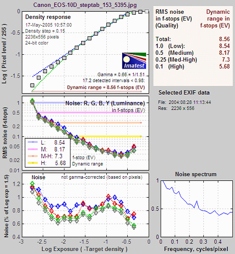
|
The
total dynamic range of
the
Canon EOS-10D is 8.6 f-stops. Total dynamic
range
improves slightly for 48-bit TIFF conversion but very little for ISO
100. But the lower noise in 48-bit TIFF conversion and ISO 100 results
in improved dynamic ranges for given quality levels.
The shape of the response curve is a
strong function of the conversion software settings. The plot on the
right
is for Canon Zoom Browser with Contrast set to Low: the transfer curve is very different from
Capture One LE, but the dynamic range is quite close— the result of slightly different noise reduction processing.
|
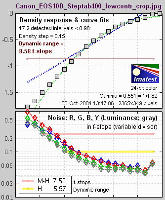 |
| Algorithm |
- Locate
the distinct zones in the image. This is done by taking the derivative
of the pixel level averaged vertically, then smoothing it, illustrated
by the light cyan spikes in the upper left plots in the above figures.
A boundary between zones is detected if this function goes above a
threshold.
The threshold is adjusted to the lowest value that gives evenly spaced,
regular intervals. This is an optimum detection
algorithm:
a lower threshold detects false boundaries (i.e., noise), while a
higher
threshold can miss valid zones.
- Find regions
of interest (ROIs) for each zone, which comprises the central 2/3 of
the
zone.
- Calculate
statistics for the ROIs, including the average pixel level and a second
order polynomial fit to the pixel levels inside the ROIs— this fit is
subtracted from the pixel levels for calculating noise. It removes the
effects of nonuniform illumination.
- Calculate
the noise in each ROI.
- Using
the average pixel values of the regions whose value is 10% below the
maximum
and above theminum, the average pixel response is fit to a mathematical
function (actually, two functions). This requires some explanation.
- Using
the average pixel values of grayscale zones for densities between
approximately
0.1 and 0.9 (omitting the extremes near white and black), the average
pixel
response is fit to a mathematical function (actually, two functions).
This
requires some explanation.
A
simplified equation for a capture device (camera or scanner) response
is,
normalized
pixel level = (pixel level/255) = k1 exposuregamc
Gamc
is the gamma of the capture device. Monitors also have
gamma
= gamm defined by
monitor
luminance = (pixel level/255)gamm
Both gammas
affect the final image contrast,
System
gamma = gamc * gamm
Gamc is
typically around 0.5 = 1/2 for digital cameras. Gamm is 1.8 for
Macintosh
systems; gamm is 2.2 for Windows systems and several well known color
spaces
(sRGB, Adobe RGB 1998, etc.). Images tend to look best when system
gamma
is somewhat larger than 1.0, though this may not hold for contrasty
scenes.
For more on gamma, see Glossary, Using
Imatest SFR, and Monitor
calibration.
Using
the equation, density = - log10(exposure) + k,
log10(normalized
pixel level) = log10( k1 exposuregamc
) = k2 - gamc * density
This is
a nice first order equation with slope gamc, represented by the blue
dashed curves in the figure. But it's not very accurate. A second order
equation works much better:
log10(normalized
pixel level) = k3 + k4 * density
+ k5 * density2
k3,
k4, and k5 are found using second order
regression
and plotted in the green dashed curves. The second order fit
works
extremely well.
|
|
Using Colorcheck
What
Colorcheck does
Colorcheck analyzes images of the widely-used
GretagMacbethTM
ColorChecker®
for tonal response (using the six grayscale patches, which have an
optical
densities from 0.05 to 1.50; a range of 1.45 = 4.8 f-stops), noise (for
the six grayscale patches), and color quality. Results for tonal
response
are similar to Imatest Q-13 program.
|
The GretagMacbeth
ColorChecker is an 8x11"
inch chart consisting of 24 patches with 18 familiar colors and six
grayscale
levels, white to black. None of the colors is completely saturated. The
quality of the chart is very high— each patch is printed separately
using
carefully controlled pigments. Patches have a smooth matte surface. It
is available from Adorama
and other dealers. A 2.25"x3.25"
mini
ColorChecker is also available.
An ideal simulated ColorChecker is shown
on the
right for sRGB color space (the Windows/Internet standard). The optical
densities (-log10(reflectivity)) of the grayscale patches on
the bottom row are shown in parentheses. One color, 18. Cyan, is out of
the sRGB gamut; hence it can't be reproduced perfectly on most monitors.
|
|

1.
dark
skin
|
2.
light
skin
|
3.
blue
sky
|
4.
foliage
|
5.
blue
flower
|
6.
bluish
green
|
7.
orange
|
8.
purplish
blue
|
9.
moderate
red
|
10.
purple
|
11.
yellow
green
|
12.
orange
yellow
|
13.
blue
|
14.
green
|
15.
red
|
16.
yellow
|
17.
magenta
|
18.
cyan
|
19.
white
(.05)
|
20.
neutral
8
(.23)
|
21.
neutral
6.5
(.44)
|
22.
neutral
5
(.70)
|
23.
neutral
3.5
(1.05)
|
24.
black
(1.50)
|
|
| What
colors are the ColorChecker? |
|
The information
supplied with
the ColorChecker is lacking. Grayscale densities (for the bottom row)
are
printed on the back of the chart. CIE xyY values (used in the familiar
xy chromaticity chart) are printed on the package and in a sheet that
comes
inside the package. The sheet also contains a set of RGB values that
corresponds
to no known color space used by photographers. It can be
ignored.
xyY values are cannot be used
directly by Imatest.
RGB values are needed to display the ColorChecker (in sRGB color space
for Website display). Also, xy chromaticity values are far from
perceptually
uniform, i.e., distances between points on the xy-plane are not
proportional
to perceptible differences between colors. (Green is greatly
exaggerated.)
Color differences are represented much better in the CIELAB color
space,
where a distance of 1 between L*a*b* values represents the minimum
perceptible
difference between colors (for relatively unsaturated colors). For
colors
on the a*b* plane, this distance is expressed by the equation,
Delta-E = sqrt( (a1*
- a2*)2+
(b1* - b2*)2 )
Delta-E is widely used to quantify
color differences.
It is the length of the lines that connect the ideal and measured a*b*
color values in the third figure, described below.
|
|
There are three
sources of
ColorChecker values. Each is slightly different.
- The
GretagMacbeth website. Two downloads are available. (1) a
ColorChecker
image, evidently in sRGB color space (though GretagMacbeth neglects to
mention this useful tidbit). (2) an Excel table of XYZ, L*a*b* and RGB
values, measured with Illuminant C (an old light source standard
similar
to D65 = 6500K and daylight). Values are closer to to Danny Pascale's
sRGB
values (~2) than to any other space.
- BruceLindbloom.com.
Contains equations and tables for converting between various RGB color
spaces as well as XYZ, xyY, and CIELAB. Click on Math.
His ColorChecker
values are based on acurate spectrophotometer measurements of a
single
sample. He has a useful ColorChecker
calculator. A rich resource.
- Danny
Pascale/BabelColor. RGB
coordinates of the Macbeth ColorChecker
presents ColorChecker values in xyY, L*a*b*, and several color spaces,
based on the same xyY values used by Gretag. He also presents
procedures
and equations for data conversion. The L*a*b* values are for D50
illumination.
I prefer Gretag's values because Illuminant C is closer to the D65
white
point of the sRGB color space.
- Bruce
Fraser, Creativepro.com. Calibrating
Camera Raw in Photoshop CS contains Bruce's ColorChecker L*a*b*
values
from his book, Real
World Color Management. I not sure what
reference
color temperature he uses. Allen
Pacheco has published a similar calibration technique.
For now, Imatest uses the
GretagMacbeth L*a*b* values
and the Pascale RGB values (close to GretagMacbeth). A future version
may
allow the source to be selected, but differences are minor.
|
|
Photographing
the target and running colorcheck
- Photograph the GretagMacbeth ColorChecker. Be sure the light is
even.
As
little as possible should come from behind the camera— it can cause
glare.
An angle of incidence of about 30 degrees is ideal for lighting. The
light
should not emphasize the texture of the chart surface— noise in
grayscale
patches in the bottom row will be measured. More that one light source
is desirable. If possible, the surroundings of the ColorChecker should
be gray or black to minimize flare light. If the lighting is uneven,
the
tops of the gray scale pixel plot (the upper left plot in the first
figure, below)
will be tilted. Tips on lighting can be found here.
-
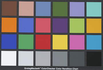 The
color checker can be photographed slightly
out of focus to minimize errors in noise measurement due to texture in
the patch surfaces. I emphasize slightly—
the dark bands between the patches should remain distinct. The texture
is quite low. If the lighting is reasonably diffuse (not a point
source),
noise from the texture should be minimal.
 - The distance at which the target is photographed is not critical.
1500
horizontal pixels is more than sufficient for all Colorcheck measurements including noise.
That is about half of the horizontal field of a 6 megapixel SLR. A
larger
chart image just slows down the calculations.
- WARNING The image should not be too large!
Images over 3000 pixels wide (6 megapixels total) can cause trouble.
The reason is that Matlab uses double precision math, which requires 8
bytes per color. Here are the numbers: A 6 megapixel camera produces 18
megabyte images in 24-bit color (6x3x1 MB) or 36 megabyte images in 48-bit color (6x3x2 MB). When this image is read into Matlab, it is converted into 144 megabytes (6x3x8
MB) of double precision data: enough to seriously slow down
calculations, especially in computers with limited memory (256 MB or
less). Be especially careful not to fill the frame with 8+ MB digital cameras.
- Save the image as a RAW file or maximum quality JPEG, then load
it on
your
computer. If you are using a RAW converter, convert to JPEG (maximum
quality),
TIFF (without LZW compression, which is not supported), or PNG.
If
you are using film, develop and scan it.
- Click on the Run Colorcheck
button in the Imatest main window.
- Open the input file using the dialog box. Imatest remembers the
directory
name of the last input file opened.
- Crop the image so a small amount of the dark boundaries
at the
left,
right, top, and bottom of the Colorchecker image are visible. There is
no harm if the boundaries are cut off as long as most of the patch area
remains; precise cropping is not critical. Click outside the
image
for no crop. The orientation does not need to be correct; Imatest will
rotate the image (in multiples of 90 degrees) to the correct
orientation.
The image on the right is representative of a good crop.
Output
The example was photographed with the Canon EOS-10D at ISO 400, and RAW
converted with Canon FVU using automatic color balance.
The
first figure: Gray scale tonal response and noise
shows graphic results derived
from
the grayscale patches in the bottom row. The results include tonal
response
and noise.

| The upper left plot shows the average density
of the
grayscale patches (black curve) and first and second order
density
fits (dashed blue and green
curves). The horizontal axis is the distance along the target. A
portion of the patches themselves are shown just above the plot. The
average
density curve is useful for diagnosing uneven lighting: the tops of
this
curve will be flat if the lighting is even. The equations for the first
and second order density fits are given in the Algorithm section, below.
The second order fit accurately matches the patches; it is used to
calculate
the corrected ideal ColorChecker values in the third figure, below. |
The upper right plot shows the density response
of the
colorchecker (gray squares) as well as the first and second order fits
(dashed blue and green
lines). The horizontal axis is Log Exposure (minus the target
density), printed on
the
back of the ColorChecker. |
| The lower left plot shows the RMS noise for
each patch:
R, G, B, and Y (luminance). The average R, G, B, and Y noise for the
gray
zones (2-5) is also reported. RMS noise is expressed in percentage of
the
difference
between the white and black patches. |
The lower right plot shows the noise spectrum
of patch
4 in the bottom row (middle gray). It contains hidden information about
signal processing, for example, an unusually rapid rolloff of noise
energy
may indicate excessive noise reduction. The ISO speed and Exposure time
from the EXIF data are displayed, if available. |
Two
precautions
when working with figures
Too
many open Figures
Figures can
proliferate
if you do a number of runs, especially SFR runs with multiple regions,
and system performance suffers if too
many
Figures are open. You will need to manage them. Figures
can be closed individually by clicking X on the upper right of
the
Figure or by any of the usual Windows techniques. You can close them
all
by clicking Close figures in the Imatest main window. |
Clicking
on Fgures during calculations
can confuse Matlab.
Plots
can appear on the wrong figure (usually distorted) or disappear
altogether.
Wait until all calculations are complete— until the Save or Imatest
main
window appears— before clicking on any Figures. |
The
second figure: noise detail
shows the density response, noise in f-stops (a relative measurement
that corresponds to the workings of the eye), noise for the third
Colorchecker row, which contains primary colors, and selected EXIF data.

| The upper left plot is the density
response
of the
colorchecker (gray squares). It includes the first and second order
fits
(dashed blue and green
lines). The horizontal axis is Log Exposure (minus the target
density), printed on
the
back of the ColorChecker. Q-13 Stepchart provides a more detailed
density response curve. |
The upper right plot shows the noise in the
third colorchecker row, which contains the most strongly colored
patches: Blue, Green, Red, Yellow, Magenta, and Cyan. In certain
cameras noise may vary with the color. Problems may be apparent that
aren't visible in the gray patches.
|
| The lower left plot shows the R, G, B, and Y
(luminance) RMS noise for as a function of Log Exposure
each patch. RMS noise is expressed in f-stops, a relative measure that
corresponds closely to the workings of the human eye. This measurement
is described in detail in the Q-13
Stepchart tour. It is largest in the dark areas because the pixel
spacing between f-stops is smallest. |
The lower right region displays EXIF data, if
available. |
The
third figure: color error
illustrates the color error in
the
device-independent CIELAB color space, where a* is the horizontal axis
and b* is the vertical axis. The small squares are the ideal (a*, b*)
ColorChecker
values, calculated by Danny
Pascale of BabelColor.
The
large circles are the (a*, b*) values of the actual measured
ColorChecker.
The numbers near the squares or circles correspond to the numbers of
the
ColorChecker patches: 1-6 are in the top row, 7-12 are in the second
row,
and 13-18 are in the third row. The numbers for patches 19-24 (the
bottom
row) are omitted because their (a*, b*) values cluster around (0, 0).

The background of the chart shows expected colors (in monitor sRGB
color
space) for L* = 0.95. It presents a reasonably accurate picture of the
hues associated with a* and b*. There is significant scatter in the
results
because the luminance (L) of the color patches (not displayed) varies
considerably.
CIELAB (often shortened to LAB) was designed to be perceptually
uniform,
meaning that the perceived difference between colors is proportional to
the distance between them, which is called delta-E. (
Delta-E = sqrt( (a2*-a1*)2
+ (b2*-b1*)2
)
). (The "-" in Delta-E is a hyphen, not a minus.) The smallest
perceptible
difference corresponds roughly to delta-E = 1. CIELAB isn't perfect in
this regard. Delta-E for the minimum perceptible color difference
increases
with distance from the origin (a* = b* = 0). But it is much more
uniform
than the popular CIE xy chromaticity diagram.
Four values are reported on the upper right.
- Mean camera saturation (%) is 100% times the average
saturation
of the camera colors divided by to the average saturation of the ideal
Colorchecker colors. The saturation of an individual color is its
distance
from the origin (sqrt(a*2+b*2)). The higher the saturation, the more intense the color. Mean
saturation
is affected by lens quality (flare light in a poor lens decreases
saturation)
and by the RAW conversion software, inside or outside the camera. Many
cameras and all RAW conversion software have have adjustments for
saturation.
It is not a strong
indicator
of image quality because it can be easily adjusted in image editors.
Images
out of the camera often look better with extra saturation (120% is not
uncommon in compact digital cameras), but a camera that boosts
saturation
runs the risk of losing detail in highly saturated objects.
- Color error (delta-E, corrected for saturation) is the
mean
(average)
distance between the camera and ideal colors, after the camera values
have
been normalized to the same average saturation as the ideal
Colorchecker.
It is a fairly significant indicator of color quality. It is mesured in
two ways:
- The mean error: the mean distance between the
measured and
ideal colors: mean( sqrt( (ameas*-aideal*)2
+ (bmeas*-bideal*)2 ) ) =
mean(delta-E).
- The root mean square (RMS) error, denoted by the Greek
letter sigma:
the square root of the mean of the squared distances between the
measured
and ideal colors: sqrt( mean( (ameas*-aideal*)2
+ (bmeas*-bideal*)2 ) ). This
number (closely related to standard deviation) gives greater weight to
large errors; it may therefore be a better overall indicator of color
accuracy.
It will be difficult to assess these numbers until a large database
of test results is available. I would characterize the mean value of
5.66
and sigma of 6.73 for the EOS-10D (above) as very good— perhaps excellent.
See the Links, below, for details on CIELAB color
space.
The fourth figure: color analysis
is an image of the ColorChecker
that
allows you to compare the actual and ideal values. It also displays
White
Balance error using the bottom row (the grayscale patches).

The outer
portion
(1) of each patch contains the ColorChecker image as photographed, The
inner portion contains the ideal ColorChecker values corrected for
exposure
(2) and uncorrected (3).
1. the outer region, is
the
patch as photographed. This corresponds to the circles in the L*a*b*
color
error plot, above.
2. the square in the
center,
is the ideal value of the patch, corrected
for the luminance of the photographed chart. The
correction
is derived from the second order fit to the gray areas, described
above.
The average luminance of zones 1 and 2 shoud be close— zone 2 may be
darker
in some patches and lighter in others. Zones 2
and 3 correspond to the
small
squares in the L*a*b* color error plot, above.
3. the small rectangle
to
the right of the central square, is the ideal value of the patch, with no
luminance correction. The luminance of zone 2 will be consistently
lighter
or darker than zone 3 for all patches, depending on the exposure.
In the above example, the ColorChecker image
1
is slightly underexposed; it is darker than the ideal uncorrected color
3.
It is also darker than the corrected ideal color 2.
This is a characteristic of this camera: it tends to darken oranges and
lighten blues and cyans. This can be seen in the above right
ColorChecker
image, which is slightly overexposed. This image of the orange-yellow
patch
(row 2, column 6) has about the same luminance as the uncorrected ideal
color 3, but is darker than the corrected ideal color. The uncorrected
ideal value 3
in the two orange-yellow images above (the example on the left and the
full chart on the right) are the same, but appear to be quite different
because of the interaction of colors in the eye— an effect that should
be familiar to artists and photographers.
This
image provides a clear visual indication of
color
accuracy. The L*a*b* color error plot provides a quantitative
indication.
The bottom of the third figure illustrates the White
Balance error, which is quantified in three ways. (1)
Saturation
S in the
HSV
color model (burgundy). S can take
on values between 0 for a perfect neutral gray and 1 for a totally
saturated
color. (2) Correlated color temperature error in Degrees Kelvin (blue),
calculated
from Color
Science: Concepts and Methods, Quantitative Data and Formulae,
by Günther Wyszecki and W. S. Stiles, pp. 2224-228. (2)
Color
temperature in Mireds (micro-reciproacal degrees) (blue),
where Mireds = 106/(Degrees Kelvin) is a more perceptually
uniform
measure.
White Balance error tends to be most visible in the gray patches
(2-5
in the bottom row). It is barely visible for S < 0.02. It is quite
serious
for S > 0.10, particularly for the lighter gray patches.
 |
The image at the bottom shows the bottom row (the
grayscale patches)
with exaggerated white
balance
error, calculated by boosting saturation S using the curve on the left,
keeping H and V constant. Low values of saturation are boosted by a
factor
of 4; the boost decreases as saturation increases. This image shows the
White Balance error much more clearly than the unexaggerated chart.
Keep it in mind that this image is worse than reality;
small
White Balance errors may not be obvious in actual photographs,
especially
in the vicinity of strongly saturated colors. |
Saving the
results
|
When the Colorcheck calculations are complete, the Save
results? dialog box appears. It allows you to choose
which results to save and where to save them. The default is
subdirectory Results
in the data file directory. You can change to another existing
directory,
but new results directories must be created outside of Imatest— using
a utility such as Windows Explorer. (This is a limitation of this
version
of Matlab.) The selections are saved between runs.
You can examine the output figures before you check or uncheck
the boxes.
After you click on Yes
or No,
the Imatest main window reappears.
The .CSV summary file contrains Excel .CSV output for the tone
level,
noise, and color calculations. It also contains some additional data,
including
EXIF data for JPEG files.
|
 |
| Algorithm |
- Locate
the regions of interest (ROIs) for the 24 ColorChecker zones.
- Calculate
statistics for the six grayscale patches in the bottom row, including
the
average pixel levels and a second order polynomial fit to the pixel
levels
in the ROIs— this fit is subtracted from the pixel levels for
calculating
noise. It removes the effects of nonuniform illumination. Calculate the
noise for each patch.
- Using
the average pixel values of grayscale zones 2-5 in the bottom (omitting
the extremes: white and black), the average pixel response is fit to a
mathematical function (actually, two functions). This requires some
explanation.
A
simplified equation for a capture device (camera or scanner) response
is,
normalized
pixel level = (pixel level/255) = k1 exposuregamc
Gamc is
the gamma of the capture device. Monitors also have
gamma
= gamm defined by
monitor
luminance = (pixel level/255)gamm
Both gammas
affect the final image contrast,
System
gamma = gamc * gamm
Gamc is
typically around 0.5 = 1/2 for digital cameras. Gamm is 1.8 for
Macintosh
systems; gamm is 2.2 for Windows systems and several well known color
spaces
(sRGB, Adobe RGB 1998, etc.). Images tend to look best when system
gamma
is somewhat larger than 1.0, though this doesn't always hold—
certainly
not for contrasty scenes. For more on gamma, see Glossary, Using
Imatest SFR, and Monitor
calibration.
Using
the equation, density = - log10(exposure) + k,
log10(normalized
pixel level) = log10( k1 exposuregamc
) = k2 - gamc * density
This is
a nice first order equation with slope gamc, represented by the blue
dashed curves in the figure. But it's not very accurate. A second order
equation works much better:
log10(normalized
pixel level) = k3 + k4 * density
+ k5 * density2
k3,
k4, and k5 are found using second order
regression
and plotted in the green dashed curves. The second order fit
works
extremely well.
- Saturation
S in HSV color representation is defined as S(HSV) =
(max(R,G,B)-min(R,G,B))/max(R,G,B).
S correlates more closely with perceptual White Balance error in HSV
representation
than it does in HSL.
The
the equation for saturation boost in the lower image of the third
figure
is S' = (1-e-4S )/(1-e-4), where e =
2.71828...
|
|
Links
- RGB
coordinates of the Macbeth ColorChecker by Danny Pascale, The BabelColor
Company, 2003 (PDF). Excellent survey of color spaces and techniques
for
calculating the RGB values of the ColorChecker.
- Bruce
Lindbloom Outstanding site with equations for converting
between color spaces and models. Slightly different L*a*b* values from
Pascale.
- Earl
F. Glynn (EFG) has an excellent description of the ColorChecker.
His Computer Lab and
Reference
Library are a goldmine of information about color, image
processing,
and related topics.
Glossary Of Terms
Aliasing
|
|
Low frequency artifacts, sometimes quite disturbing, that appear when signal energy above the Nyquist frequency
reaches the digital sensor. Color aliasing in Bayer sensors can be
particularly troublesome. "Moire fringing" is a type of aliasing. |
|
Aperture
|
|
The circular
opening at
the center of a lens that admits light. Generally specified by the
f-stop,
which is the focal length divided by the aperture diameter. A large
aperture
corresponds to a small f-stop. This can confuse beginners. |
Bayer sensor
|
|
The
sensor pattern used in most digital cameras, where alternate rows of
pixels are sensitive to RGRGRG and GBGBGB light. (R = Red; G = Green; B
= Blue.) The sensor output has to be converted into a standard file
format (for example, JPEG, TIFF, or PNG), where each pixel represents
all three colors, by a RAW converter (in the camera or computer), which
performs a "de-mosaicing" function. The quality of RAW converters
varies: separate converter programs run in computers can provide finer
results than the converters built into cameras. That is one of the
reasons that RAW format is recommended when the highest image quality
is required.
In Foveon sensors (used in Sigma cameras), each pixel site is sensitive
to all three colors. Foveon sensors are less susceptible to color
aliasing than Bayer sensors; they can tolerate greater response above Nyquist with fewer ill effects. |
|
Chromatic
aberration
(CA)
|
|
A lens
characteristic that
causes different colors to focus at different locations. There are two
types: longitudinal, where different colors to focus on different
planes,
and lateral, where the lens focal length, and hence magnification, is
different
for different colors. Lateral CA is the cause of a highly visible
effect
known as color fringing. It is worst in extreme wide angle, telephoto,
and zoom lenses. Imatest SFR
measures lateral CA (color fringing). See Chromatic
aberration and Eliminating
color fringing. |
|
Cycles,
Line Pairs,
Line Width
|
|
A Cycle is the
period a
complete repetition of a signal. It is used for frequency measurement.
A Cycle is equivalent to a Line Pair. Sometimes Line Widths are used
for
historical reasons. One Line Pair = 2 Line Widths. "Lines" should be
avoided
when describing spatial frequency because it is intrinsically
ambiguous.
It usually means Line Widths, but sometimes it's used (carelessly) for
line pairs. |
|
Density
(Optical density)
.
.
|
|
The
amount of light reflected or transmitted by a given media, expressed on
a logarithmic (base 10) scale. For reflective media (such as
photographic
or inkjet prints), density = –log 10(reflected light/incident
light). For transmissive media (such as film), density = –log 10(transmitted
light/incident light).The higher the density, the less light is
transmitted
or reflected. Perfect (100%) transmission or reflection corresponds to
a density of 0; 10% corresponds to a density
of 1; 1% corresponds to a density of 2, etc. Useful equations:
1 f-stop (1 EV)= 0.301 density units; 1 density unit = 3.32 f-stops.
����������������� When an object is photographed,
Log Exposure = –density
+ k. (Constant k is generally ignored.) |
Dynamic
range
|
|
The range of exposure (usually measured in
f-stops) over which a camera responds. Also called exposure range. Practical dynamic range is
limited by noise, which tends to be worst in the darkest regions.
Dynamic range can be specified as total range over which noise remains under a specified level— the lower the
level, the higher the image quality. Dynamic range is measured by Q-13 Stepchart, using transmission
step charts. |
Exposure value (EV) |
|
A measure of exposure, where a change of 1 EV means doubling or halving exposure. Often synonymous with f-stop. By definition, 1 EV is a 1 second exposure at f/1.0. |
|
f-stop
.
|
|
A
measure of the a lens's
aperture (the circular opening that admits light). A a change of "one f-stop" implies doubling or halving
the exposure. This is the synonymous with a change of 1 EV.
F-stop = focal length / aperture diameter. The notation, "f/8," implies (aperture diameter = ) focal length/8. The larger the f-stop,
the
smaller the aperture. F-stops are typically labeled in the following
sequence,
where the admitted light decreases by half for each stop: 1, 1.4, 2,
2.8, 4,
5.6, 8, 11, 16, 22, 32, 45, 64, ... Each f-stop is the previous f-stop
multiplied by the square root of 2. |
|
Gamma
|
|
Exponent
that relates pixel levels in image files to brightness of the monitor
or
print. Most familiar from monitors, where luminance = pixel levelgamma.
A camera (or film + scanner) encodes the gamma so that pixel level =
brightness(camera
gamma). Imatest reports
camera gamma. Gamma is equivalent to contrast. The
reason can be observed in traditional film curves, which are
represented
on logarithmic scales (typically, density (log10(absorbed
light)
vs. log10(exposure)). Gamma is the average slope of this
curve
(excluding the "toe" and "shoulder" regions near the ends of the
curve),
i.e., the contrast. See Kodak's
definition in Sensitometric
and Image-Structure Data. For more detail, see the
descriptions
of gamma in Using Imatest SFR
and Monitor
calibration.
Confusion
factor: Digital cameras output may
not follow an exact gamma (exponential) curve: A "tone reproduction curve" (an "S" curve) may be superposed on the gamma curve to extend dynamic range
while
maintaining visual contrast. Such a curve boosts contrast in middle tones while reducing it in
highlights
and shadows. The tone reproduction curve may also be adaptive:
camera gamma may be increased for low contrast scenes and decreased for
contrasty scenes. This can affect the accuracy of SFR measurements. But
it's not a bad idea for image making: it's quite similar to the
development
adjustments (N-1, N, N+1, etc.) Ansel Adams used in his zone
system. |
|
MTF
|
|
Modulation
Transfer Function.
Another name for Spatial Frequency Response (SFR). Indicates the
contrast
of a pattern at a given spatial frequency relative to very low spatial
frequencies. See Sharpness and Understanding
image sharpness and MTF curves. |
|
MTF50
|
|
The spatial
frequency where
image contrast is half (50%) that of low frequencies. MTF50 is an
excellent
measure of perceived image sharpness because detail is diminished but
still
visible, and because it is in the region where the response of most
cameras
is declining most rapidly. It is especially valuable for comparing the
sharpnesss of different cameras. See Sharpness
and Understanding
image sharpness and MTF curves. |
Noise
|
|
Random variations of image luminance arising from grain in film or electronic perturbations in digital sensors. Digital sensors suffer from a variety of noise mechanisms,
for example, the number of photons reaching an individual pixel. Noise
is a major factor that limits image quality. In digital sensors it
tends to have the greatest impact in dark regions.
Noise is measured as an RMS value (root mean square; an indication of noise power, equivalent to standard deviation, sigma).
It is usually expressed in volts, millivolts, or pixel levels (in a
digital file). In Q-13 and Colorcheck, noise is converted
to relative luminance units (f-stops), which provide a more meaningful indication of its visual impact.
The visual impact of noise is also affected by the size of the image—
the larger the image (the greater the magnification), the more
important noise becomes. Since noise tends to be most visible at low
spatial frequencies, the noise spectrum has some importance (though it
is difficult to interpret). |
|
.
.
Nyquist
frequency
|
|
The
highest
spatial frequency where a digital sensor can capture real information.
Nyquist frequency
fN = 1/(2 * pixel
spacing). Any information above fN that reaches the
sensor
is aliased to lower
frequencies,
creating potentially disturbing Moire patterns. Aliasing can be
particularly
objectionable in Bayer sensors in digital cameras, where it appears as
color bands. The ideal lens/sensor system would have MTF = 1 below
Nyquist
and MTF = 0 above it. Unfortunately this is not achievable in optical
systems;
the design of anti-aliasing (lowpass) filters always involves a
tradeoff
that compromises sharpness.
A large MTF
response above
fN
can indicate potential problems with aliasing, but the visibility of
the
aliasing depends on whether it arises from the sensor (worse) or sharpening
(not as bad). The
Nyquist sampling theorem and aliasing contains a complete expositon. |
Raw files |
|
RAW files are the unprocessed output of digital camera image sensors. For Bayer sensors, each RAW pixel represents a single color in RGRGRG, GBGBGB, ... sequence. To be converted into usable, standard file formats (TIFF, JPEG, etc.), raw files must be run through a RAW converter (de-mosaicing) program. RAW converters perform additional functions: they add the gamma curve and often an additional tonal response curve, and they reduce noise and sharpen the image. This can interfere with some of Imatest's measurements.
The only way you can be sure an image file faithfully resembles the RAW file— that it has no sharpening or noise reduction— is to read a RAW file into Imatest and convert it to PPM format using Dave Coffin's dcraw. |
|
Resolution
|
|
The first thing
to remember
about resolution is that it has no unique definition; it can be defined
in many ways, some of which can be quite misleading. (It is almost as
abused
as the word "holistic.") In a generic sense, resolution refers to any
measurement
of an imaging system's ability to resolve fine detail. For traditional
film cameras, it usually refers to vanishing resolution— the
highest
spatial frequency where the pattern on a bar chart (usually the USAF
1951
chart) was visible. Since this tells you where detail
isn't,
it isn't a very good indicator of perceived sharpness. The pixel per
inch
(PPI or DPI) rating of a scanner is often called its "resolution." This
can be highly misleading. For example, inexpensive flatbed scanners
can't
come close to resolving the detail of decent film scanners with the
same
PPI rating. I prefer MTF50 as a measure of resolution. For more on
resolution,
see Pixels,
Images,
and Files and Lens
testing (the old-fashioned way). |
|
SFR
|
|
Spatial
Frequency Response.
The response of a system to a pattern at a given spatial frequency,
i.e.,
the contrast. SFR is measured relative to contrast at very low spatial
frequencies. It is expressed as a fraction or percentage. Synonymous
with
MTF. See Sharpness and Understanding
image sharpness and MTF curves. |
|
Sharpening
|
|
Signal
processing applied
to digital images to improve perceived image sharpness. It can be
applied
in the camera or in post-processing (image editing). Virtually all
digital
images benefit from some degree of sharpening, but images can be
oversharpened,
resulting in highly visible "halos" (overshoot) near edges. See Sharpening. |
|
Standardized
sharpening
|
|
An algorithm
used by Imatest
that allows cameras with different amounts of sharpening to be compared
fairly. With standardized sharpening, all cameras have a similar amount
of overshoot (around 5%) near edges. Without it, built-in sharpening
strongly
affects test results, giving oversharpened cameras an unfair advantage.
Results with standardized sharpening should not be used for comparing
different
lenses on the same camera. See Standardized
sharpening. |
Troubleshooting
Installation
Update installations usually do not require an uninstall of the previous
version, but if you encounter difficulties you may want
to uninstall and reinstall Imatest. The Uninstaller is accessable from the Start menu
(Start, All programs, Imatest,
Uninstall) or from the Add
or Remove Programs function of the Control Panel. The Uninstaller
gives you the option of keeping or removing the Matlab runtime library
archive,
Imatest-lib.exe. (Keep is the default;
you have to check the box to remove it.) Keeping it speeds up reinstallations.
Remove it only if you don't plan to reinstall Imatest.
Runtime errors
SFR run does not complete as expected: The contents of the imatest.ini file in the Imatest installation folder may contain clues to the problem. If you encounter this,
- Send an e-mail to Imatest support with imatest.ini attached. In English language installations the file name is C:\Program files\Imatest\imatest.ini. This will help us diagnose the problem.
- In the Imatest main window, click on File (in the toolbar), Reset defaults. This empties imatest.ini.
For other Imatest errors that shut down the DOS window,
-
Run Imatest from the Imatest folder (C:\Program files\Imatest in English
installations) by double-clicking Imatest_diagnostics
 .
This keeps the DOS window open after Imatest terminates so you can view
the error message.
-
E-mail the error message to Imatest support.
An attached screen image of the DOS window is sometimes helpful. Use
Alt-PrintScreen to copy the image into the clipboard. Paste it into an
image editor (IrfanView works well),
save it as a GIF file (TIFF is too large), then attach it to your
e-mail.)
Bugs and all that
The following message appears several times in the DOS window when
you try to save data.
Function
'get_param' is not implemented in standalone mode.
This seems to have no effect on the saved images, and it's rarely
visible since the DOS window remains in the background. Matlab has described the problem, to be fixed in a future release, here.
The Open files dialog box cannot be resized. This is a bug in Matlab
Release 13. It worked in Release 12, and was supposed to be fixed in Release
14. It isn't, and Release 14 has some other issues (it's huge and slow).
More documentation
Instructions for individual Imatest
modules can be found in the Imatest Documentation
page.
Contact
Imatest contact information
For general support questions, write
 . .
For questions about registration, sales, and related issues, write Henry Koren,
 . .
For questions about the Imatest program, algorithms, instructions, or website content, write Norman Koren,
 ,
or phone him at 303-546-6639 (USA Mountain time). ,
or phone him at 303-546-6639 (USA Mountain time). |
|
| You can usually open your e-mail client by clicking on the e-mail link on the left. If it doesn't work, enter it manually. |
|
| Imatest was founded in Boulder, Colorado in 2004 to develop software for testing digital camera image quality and lens sharpness using simple, widely-available targets. It is a spinoff of the highly informative digital photography website, www.normankoren.com. |
Norman Koren, the founder and president, has been involved with photography since 1964. He has a BA in physics from Brown University and an MA in physics from Wayne State University. His previous career in magnetic recording technology has provided him with an outstanding background for image quality analysis.
Henry Koren, the systems programmer, has been working in website design, e-commerce, and general programming since 1998. |
|
Travel plans
Norman is planning to visit India, December 5-30, where he'll be frequenting Internet cafes. He may be a little slow responding to e-mails during his travels.
Future trips: Jan. 2005: San Jose, CA (Electronic Imaging conf.), Feb. 2005: Los Angeles/Southern California, Mar. 2005: Portland, OR (SPE conf.) |
|
Change Log
Imatest release history
Imatest change log (release notes)
| Date |
Release |
Description |
| Dec. 3, 2004 |
Imatest 1.2.5 |
Issues a warning for uneven illumination in Colorcheck. Displays average R, G, B, and Y noise levels in Q-13 Stepchart. Fixes a bug that caused Imatest to crash when an attempt is made to save a figure that hasn't been created. |
| Nov. 16, 2004 |
Imatest 1.2.3 |
Print test Gamut maps have been enhanced to display lines of constant hue. |
| Nov. 14, 2004 |
Imatest 1.2.2 |
Print test now displays La*b* saturation maps, which illustrate gamut with great clarity. Print test is now complete, but it will retain beta status for two weeks. It is available to all users. The Colorcheck La*b* color error plot now displays the color space gamut limits as a gray line in the background. |
| Nov. 4, 2004 |
Imatest 1.2.1 |
Fixes a rare glitch in dynamic range calculations. Allows the Chromatic Aberration figure to be turned off. Increases the size of the image used for cropping. Includes a beta version of the new Print test module, available only to registered users. Documentation will be available in a few days. |
| Oct. 24, 2004 |
— |
A new page has been added to the website: How to test lenses with Imatest. The description of SFR figures has been divided into three pages: MTF (Sharpness) plot, Chromatic Aberration, Noise, and Shannon Capacity plot, and Multiple ROI (Region of Interest) plot |
| Oct. 17, 2004 |
Imatest 1.2 |
RAW files are supported for a large number of digital cameras using Dave Coffin's dcraw program. Files are converted with minimal signal processing— no sharpening or noise reduction. This allows the true performance of cameras and the behavior of raw converters to be analyzed.
Chromatic Aberration is now measured as percentage of the distance from the image center. This is an improvement over area in pixels because CA tends to be proportional to that distance. The new measurementand is relatively independent of camera pixel count and measurement location.
A checkbox on the main window allows you to turn off automatic expansion of the figures for high resolution screens (>1280 pixels wide). The smaller figures are better for posting on the web. |
| Oct. 12, 2004 |
Imatest 1.1.3 |
SFR regions of interest (ROIs) are now saved between runs. B&W images are handled better by SFR: A message is displayed indicating that Chromatic Aberration can't plot, and Noise/Shannon capacity plots properly. |
Oct. 7, 2004
|
Imatest 1.1.2
|
Fixes a memory problem that slowed repeated SFR runs.
|
Oct. 6, 2004
|
Imatest 1.1.1
|
Lighter grid lines make plots
far more legible. SFR output has been simplified for clarity. Dynamic
range information is displayed more clearly on Q-13 Sepchart.
|
|
Sept. 28, 2004
|
Imatest
1.1
|
Greatly expands noise and
dynamic range
calculations in Q-13 Stepchart and noise
calculations in Colorcheck. Noise measurements
in f-stops have been added to both programs. These are relative measurements, which
correspond closely to the workings of
the eye. Q-13 Stepchart now calculates total dynamic range (using a
more sensitive detection algorithm) as well as noise-limited dynamic
ranges for several quality levels. Colorcheck now includes noise
measurements for the third Colorchecker row, which includes Blue,
Green, Red, Yellow, Magenta, and Cyan.
In evaluation mode, multiple region SFR runs now count as two runs
(even if more than two regions are selected).
|
Sept. 11, 2004
|
Imatest
1.0.3
|
Improves compatibility with
48-bit color files.
|
| Sept. 7, 2004 |
Imatest 1.0.2 |
Fixes some registration/activation issues. Not
needed if you were able to register 1.0. |
| Sept. 6, 2004 |
Imatest 1.0.1 |
| Sept. 4, 2004 |
Imatest 1.0 |
The first release! A number of improvements
have been made since the final Beta version. Q-13 now displays camera
dynamic range when run with transmission step targets (the reflective
Q-13 has insufficient contrast to measure the dynamic range of digital
cameras.) Colorcheck now displays the color temperature error (in
degrees K and mireds) of the Colorchecker gray patches. A bug was fixed
that caused SFR to always calculate the MTF for the same color channel. |
|
Beta versions |
| August 14, 2004 |
Beta 1.5.13 |
Some small enhancements, including a drop-down help menu with
the beginnings of the purchase/registration dialog. |
| August 12, 2004 |
Beta 1.5.12 |
A few small fixes. Change directory in the Save windows now
works correctly. |
| August 11, 2004 |
Beta 1.5.10 |
Contains a speedup
for runs where the ROI is repeated— it allows you to omit the requests
for input data and save information, which is assumed to be repeated.
The shortcut for installations where other Matlab versions are present
is changed (see Troubleshooting, below). Excel .CSV output has been added to
the Colorcheck module. |
| August 9, 2004 |
Beta 1.5.7 |
Incorporates several suggestions from Q. Tuan Luong. Multi-region
runs now display two vertical axes for MTF and a box with a summary of
the results— a weighted MTF that can be used as an overall sharpness
figure. SFR Cycles per (pixel, mm, inch) plot settings are saved
between runs. Multi-region output has been documented here. |
| August 7, 2004 |
Beta 1.5.6 |
Fixes a bug in the SFR binning algorithm that caused
occasional crashes. It displays numeric results on the multiple ROI
plots. Digitalcamerainfo.com,
a new digital camera review site from the creators of Camcorderinfo.com, has become
the first site to use Imatest for its tests. |
| August 3, 2004 |
Beta 1.5.5 |
Corrects some problems with multiple ROI selection and
improves some details of the Excel .CSV output files. |
| August 1, 2004 |
Beta 1.5.4 |
Has the exact equations for converting between sRGB, XYZ, and
Lab color spaces. Beta 1.5.3 adds Adobe RGB (1998) files to Colorcheck.
A problem with creating imatest.ini has been solved. No additional
features are planned for the product release— just refinements and bug
fixes. More documentation is coming. |
|
| July 29, 2004 |
Beta 1.5.2 |
Has some minor fixes and small improvements in the multiple
region plots. |
| July 27, 2004 |
Beta 1.5 |
produces plots of MTF50 (without and with standardized
sharpening) and rise distance as a function of distance from the center
of the frame for images where multiple regions have been selected. This
is a big advance— the results for several locations are summarized in
two figures. Full documentation is forthcoming. |
| July 26, 2004 |
Beta 1.4.6 |
Stores and recalls settings, including directories for
reading and saving images, SFR plot settings, and save selection. This
is a major convenience.Settings are stored in imatest.ini, which is a
simple, readable ASCII file. |
| July 18, 2004 |
Beta 1.4.4 |
Has some improvements in ROI selection, displays MTF30
instead of MTF20 (minor change) and adds standard deviation (sigma) to
the L*a*b* color error. I'll be traveling until July 24. I've left some
old versions (below) as a backup. |
| July 17, 2004 |
Beta 1.4.2 |
Fixes some font size problems with 1600x1200+ screens. The
OK/Cancel buttons have been switched in some dialog boxes: OK (yes) is
always on the left. |
| July 16, 2004 |
Beta 1.4.1 |
Now allows you to select several regions of interest (ROIs)
in SFR instead of just one. This makes it convenient to test sharpness
from the center to the edge, etc. ROIs are now saved. If you run SFR on
an image with the same pixel dimensions as the previous image, SFR will
ask you if you want to use the same ROIs. This can speed up repeat
runs, for example, when the same image is used to test a lens at
several f-stops. There is still much to be done with the output—
combining the results of multiple runs. |
| July 12, 2004 |
Beta 1.3.4 |
Has simplified SFR output by plotting omitting the LW/PH MTF
Figure (as default) and removing the Shannon capacity and noise
spectrum plots from the Chromatic Aberration Figure (also as default).
These plots can be restored by means of a checkbox. The installer does
somewhat more rigorous checking for installed libraries. |
| July 11, 2004 |
Beta 1.3.3 |
Fixes the font size problem in the GUI windows— All fonts
should now be set properly by the font size box. It also addresses some
Install/Uninstall issues. Windows XP should be OK, but there may still
be problems with 98. |
| July 8, 2004 |
Beta 1.3.1 |
Changes the definition of camera gamma so pixel level =
exposure(camera gamma). It corrects some Q-13 display
issues: the first zone is now number 1. |
| July 5, 2004 |
Beta 1.3.0 |
The installer has arrived. Installation is now simple— just
double-click on Imatest-[version].exe and answer the questions—
mostly click Next >. There is a new password. The old
version will remain on this page for a few days— until the Installer
has been tested on all versions of Windows (98, 2000, and ME, in
addition to XP). |
| July 2, 2004 |
Beta 1.2.6 |
Has an option for an Excel .CSV plot of (cycles/pixel, LW/PH,
MTF, MTF(corr)). The aerial MTF50 is now called "ideal megapixels." |
| July 1, 2004 |
Beta 1.2.5 |
Includes estimates of aerial MTF50 (half-contrast frequency
in megapixels) in addition to linear MTF50 (in cycles/pixel and LW/PH). |
|
| June 26, 2004 |
Beta 1.2.3 |
Incorporates several small improvements, including the
ability to select the standardized sharpening radius. Because the
directory structure has been changed to conform to the final (I hope)
release, I recommend the following steps for upgrades from Beta 1.2.2
or earlier. Download and uncompress bothimatest.zip
and imextras.zip. Then double-click on
install2.bat (or install98.bat for Windows 98). This should put the
files in their correct folders. |
| June 24, 2004 |
Beta 1.2.2 |
Has better zone detection in Q-13. Beta 1.2.1. Q-13 analyzes
several step charts in addition to the Q-13, including transmission
charts from Kodak and Stouffer. These charts are valuable for testing
dynamic range and performance in scanners and digital cameras.
Colorcheck displays the average R, G, B, and Y noise for the gray
patches. |
| June 22, 2004 |
Beta 1.2.0 |
Allows Colorcheck and Q-13 images to be cropped. This makes
it easy to analyze Colorchecker images in the "Davebox" images in imaging-resource.com.
48-bit color files are now supported. Colorcheck and Q-13 request the
title of the run (which defaults to the input file name). |
| June 17, 2004 |
Beta 1.1.3 |
Corrects some cropping issues with Colorcheck and reports
gamma in a consistent manner for all modules (generally in the vicinity
of 2). Where "Oversharpening" was a negative number, it is now reported
as "Undersharpening." The Imatest
forum for posting questions and responses is now working. |
| June 10, 2004 |
Beta 1.1.1 |
Has choice of small, normal, and large fonts to cover a wider
range of screen resolutions. Plot size is increased for 1600x1200 or
larger screens. Mean saturation and color error have been added to the
Colorcheck L*a*b* color error plot. If new EXIF data is present, data
derived from previous EXIF entries is cleared. Clipping warning message
boxes and tooltips have been added. |
|
| May 28, 2004 |
Beta 1.1.0 |
Has a new input window for SFR that allows output to be set
to cycles per mm, along with numerous other settings. It also allows
the output font size to be reduces. I'll be on the west coast from May
29-June 8. I may be a little slow responding. |
| May 23, 2004 |
Beta 1.0.6 |
Numerous small improvements in displays. At Lee Jalovec's
suggestion, I'll increment the last number of the release version (now
.6 in 1.0.6) for every build, no matter how minor. That will
make it easier to keep track. |
| May 18, 2004 |
Beta 1.0.5 |
Corrects a number of Colorcheck issues and has a new L*a*b*
color error diagram. |
| May 13, 2004 |
Beta 1.0.4 |
Some minor bug fixes and refinements. I discovered it's
important to copy all .fig files to subdirectory bin
(C:\Program files\Imatest\bin ).The Change directory box inthe Imatest
main window was removed. Imatest modules now remember the lastdirectory
used. There are new versions of install2.bat and install98.bat.ALL.fig
files must be copied to subdirectory bin of the Imatest directory (to
C:\Program files\Imatest\bin ) for Imatest to work reliably. |
| May 9, 2004 |
Beta 1.0.3 |
A number of small improvements, including calculation of
Shannon capacity for several signal levels, representing several image
contrast levels. I've radically updated the documentation, but there
are still plenty of loose ends. The installer is still on the way. |
|
| April 29, 2004 |
Beta 1.0 |
I released Beta 1.0, which has a GUI— graphics user
interface. It is better than the old version in every way, and it has
incorporated most of the improvements and bug fixes suggested by the
Beta testers (thanks to all of you). I have to reread my e-mails to see
if I missed any. It includes two new modules— ColorCheck for analyzing
the GretagMacbeth ColorChecker, and Q-13 for the Kodak Q-13 gray scale.
These are far from complete and not yet properly documented. |
| April 21, 2004 |
Beta 0.07 |
Now based on Matlab Release 13 (version 6.5.1). Must be
reinstalled from scratch, not as an upgrade. It will take two or three
days for the documentation to catch up. The GUI won't be ready for a
while. The Chromatic Aberration calculation has been corrected. Gamma
has been inverted: It now defaults to 2 (less confusing). Noise
calculations, noise spectrum, and an approximate Shannon capacity have
been added. There have been a number of interface improvements— but
the BIG one— the GUI— is two or three weeks away. I am now
using Matlab Release 13, version 6.5.1. It has different libraries from
the previous version (6.1). The program must be reinstalled from
scratch— not as an upgrade. |
| April 12, 2004 |
|
I will be adding a proper graphic user interface (GUI) and an
installer.
Imatest will resemble a commercial program when these are finished.
Then I need to set up an e-commerce host with an affiliate program, a
means of limiting the evaluation version and registering the full
version, and a bulletin board. |
|
| March 31, 2004 |
Beta 0.06 |
Now includes a Chromatic Aberration plot. Asks whether you
want to save the results of the run (so your folders don't get
cluttered with bad results). |
| March 27, 2004 |
Beta 0.05 |
Sharpening radius is adjusted to give good results for
blurred edges. |
| March 23, 2004 |
Beta 0.04 |
Box that requests another SFR run gives option of using same
image. Many small refinements. |
| March 22, 2004 |
Beta 0.03 |
Region of Interest (ROI) selection of digital camera images
now functions properly. Some data is "sticky:" it remains unchanged
between successive runs. Many small improvements have been made on the
user interface. |
| March 20, 2004 |
Beta 0.02 |
Files are now written for use with Microsoft Excel. |
| March 17, 2004 |
Beta 0.01 |
First Beta release. |


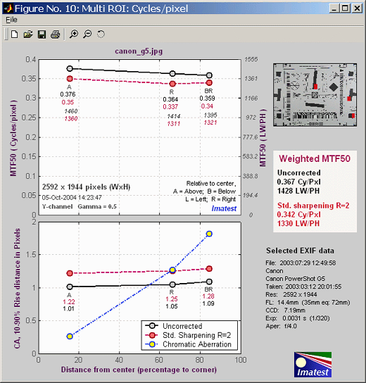

 Download the Print test pattern,


 Although
MTF can be estimated from images of a sine pattern (see the page on
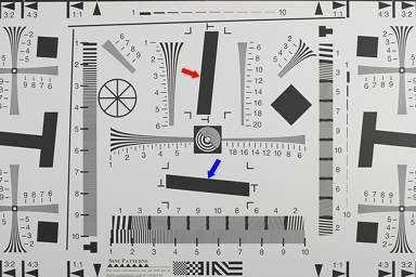


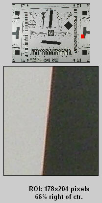




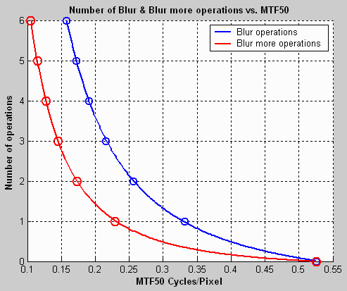

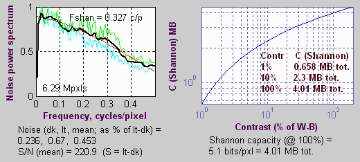


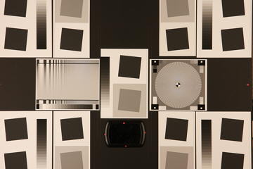

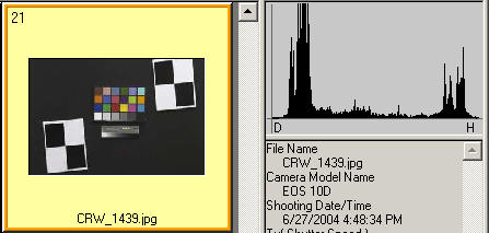


 Plot controls which results are plotted. Plot settings are saved between runs. The boxes to the right of "Cycles per" control the x-axis display. You can choose between Cycles per pixel (the default), Cycles per inch, or Cycles per mm. If you choose Cycles per inch or mm, you must enter a number for the pixel size— either in pixels per inch, pixels per mm, or microns per pixel. An example is shown below for a plot in Cycles per mm for the Canon EOS-10D, which has a pixel spacing of 7.4 microns. If you omit this, the x-axis will be displayed in Cycles per pixel.

 The most important of the Imatest SFR figures, shown on the right, contains the average edge profile on top and MTF (spatial frequency response) on the bottom. (Input-related data on the right of the figure is omitted here.)



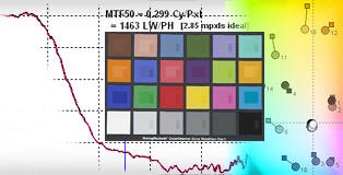

 does not work during region selection. Imatest mistakely assumes you are trying to select the entire image. To enlarge the image (to view the crop area more clearly), maximize it by clicking on the square next to the upper right corner of the Window.


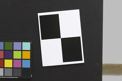


 The Imatest SFR data window, shown on the right, appears after the Region of
Interest (ROI) has been selected, unless Express mode has been chosen.
It appears only once during multiple ROI runs. Succeeding runs have the
same entries except for Crop location.
All input fields are optional. Most of the time you can simply click


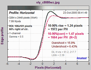


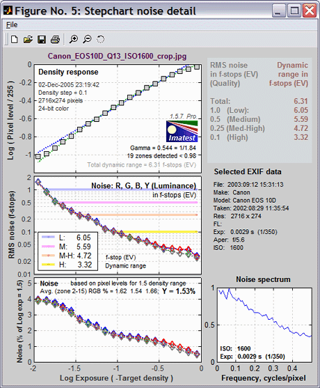


 For
flatbed scanners, you can simply lay the step chart down on the glass.
Stray light shouldn't be an issue, though there is no harm in keeping
it
to a minimum. 35mm film scanners may be difficult to test since they
can
only scan 36mm segments. (Most transmission targets are longer.) For
scanners
specified as having Dmax greater than 3, the chart of choice is the


 The
color checker can be photographed slightly
out of focus to minimize errors in noise measurement due to texture in
the patch surfaces. I emphasize slightly—
the dark bands between the patches should remain distinct. The texture
is quite low. If the lighting is reasonably diffuse (not a point
source),
noise from the texture should be minimal.