Introduction
| The image sensor noise model is the heart of the Simatest Camera/Image Signal Processing (ISP) simulator. It enables camera performance (SNR, image information metrics, and more) to be characterized and simulated for a wide variety of conditions, especially low illumination levels, or equivalently, high Exposure Indices (ISO speeds). |
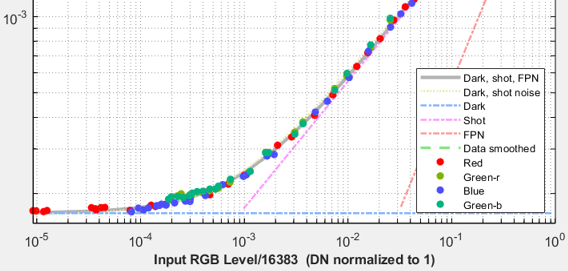
Noise vs. Digital Number, DN (Photon Transfer Curve) from raw image (Noise plot 10 from Color/Tone)
This post shows how to measure, model, and use image sensor noise measured from raw images to
- model complete image system performance with Simatest, Imatest’s Imatest Camera / Image Signal Processing (ISP) simulator, which allows camera systems and ISP to be designed and tested in software before a prototype is built.
- measure image sensor dynamic range, which is generally higher than camera dynamic range, which is limited by stray light (flare, veiling glare) from the lens.
Raw images (undemosaiced and unprocessed) are used to measure image sensor noise because they can take advantage of a remarkable property of image sensors.
|
Noise vs. normalized Digital Number, DN, for JPEG image
The noise in a uniformly illuminated region (i.e., a flat patch) of a raw image is a function of its mean Digital Number, DN, independent of the color. That means that the noise and SNR (Signal-to-Noise Ratio) for all channels fits a single well-defined curve, as shown above-right. Once image processing has been applied, as it has in the JPEG file of the same image capture on the right, the curve becomes jumbled and unusable. |
Experimental technique
Experimental technique is described in detail elsewhere, primarily in Dynamic Range, and also in Color/Tone Interactive. Briefly,
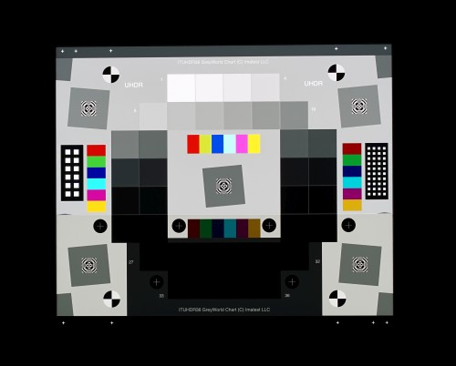
- Transmissive dynamic range test charts are recommended because they have a larger tonal range than reflective charts. A backlit 36-patch Dynamic Range chart, shown on the right, is used for the examples on this page.
- Frame the chart so it occupies the central portion of the image, typically less than shown on the right, unless the camera has extremely low resolution. This avoids problems that can arise from lens vignetting (light falloff) and with strongly distorted (fisheye) images. The image of the chart does not need to be more than 800 pixels high (less is OK for low resolution images). The chart may be moved slightly off center if needed to reduce reflections from the brightest region (top row) on the darkest regions.
- Set the gain to the minimum allowed value. For consumer cameras, this means the minimum ISO speed (Exposure Index), If the gain is larger, the image may saturate before the the sensor is saturated, and it will not be possible to obtain sensor saturation capacity and related results.
- Photograph the chart in a totally darkened environment. Any stray light reflected from the front of the target will distort the results. The surroundings of the chart and camera should be kept as dark as possible to minimize flare light. Take care to avoid reflections.
- Expose carefully, taking care to avoid overexposure, which is common in charts with dark backgrounds. An overexposed image is defined as having several (≥ 2) clipped patches, resulting in excessive stray light that can fog the image — falsely increasing the dark signal and distorting SNR and hence dynamic range measurements. Several exposures are recommended — at least one properly exposed (with one patch clipped) and one strongly underexposed (by about 3-4 f-stops — 1/8 to 1/16 the nominal exposure) to obtain a good estimate of dark signal and noise.
- save the image in a 16-bit (or more) raw format. We obviously don’t recommend JPEG files.
Enabling the Sensor Noise Model
To enable the sensor noise model for color/tone noise analysis of Bayer RAW images:
-
Open Imatest and go to the Settings menu at the top of the window.
-
In the left sidebar, navigate to General Settings > Calculation.
-
Under the Calculation section, find the option labeled “Use sensor noise model for color/tone noise analysis of Bayer RAW images”.
-
Toggle the switch to the On position (blue) to enable the sensor noise model.
-
Click Save in the lower right corner to apply your changes.
This setting allows Imatest to estimate temporal and fixed pattern noise using a three-component sensor noise model.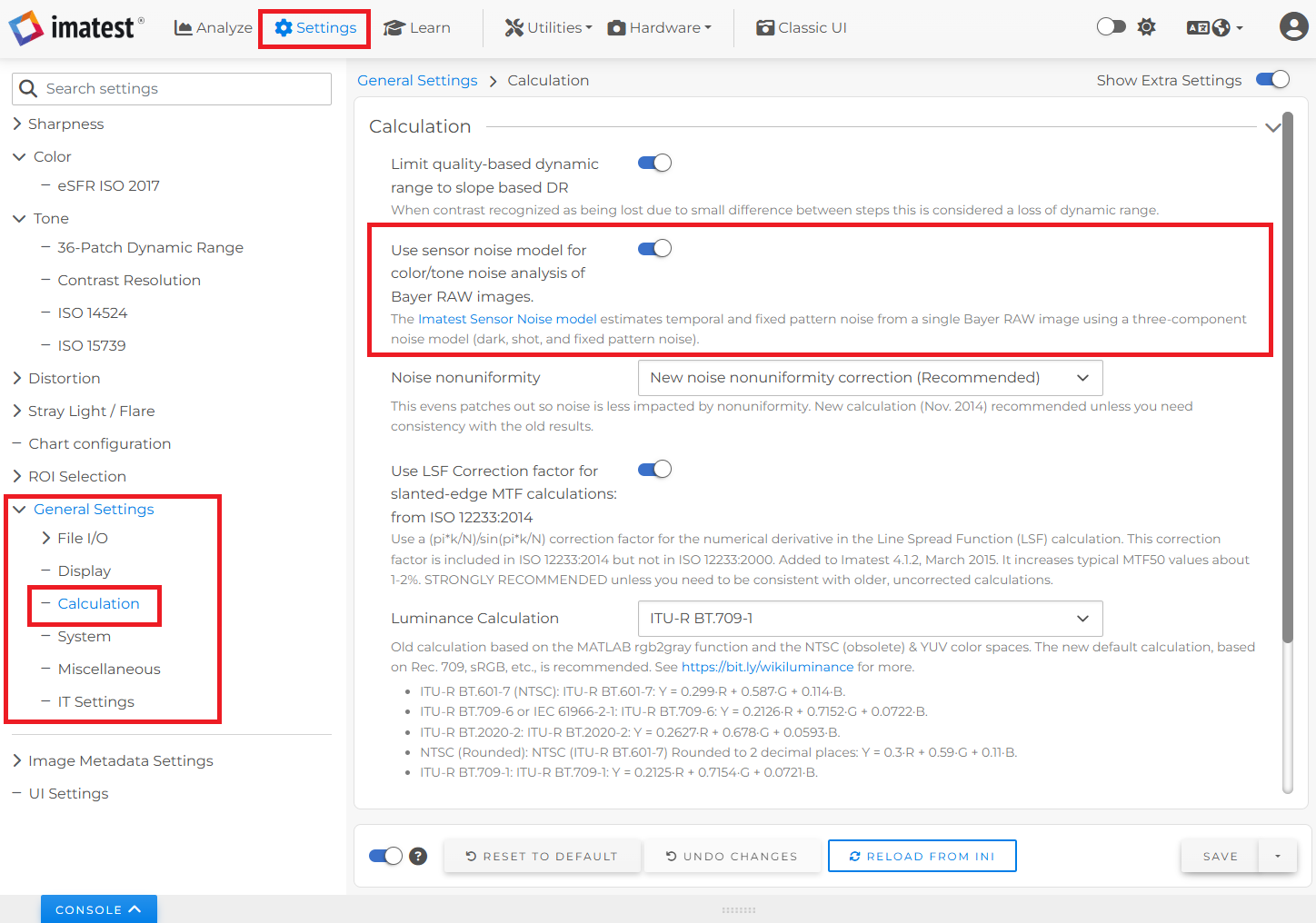
Raw file types
Imatest supports two types of RAW file.
- Commercial RAW files, from high-quality consumer cameras. These files are identified by standard extensions (ARW, CR2, NEF, RW2, etc.). They contain header data and are usually packed so that m pixels are stored in n bytes. There are normally processed (demosaiced) using LibRaw, which can be set to keep the file undemosaiced.
- Binary RAW files from development systems. These files rarely contain headers or EXIF metadata, and pixels are usually stored in 1 or 2 bytes. They identified by custom extensions defined by the user and are processed using Imatest’s Generalized Read Raw function.
Read commercial raw files with LibRaw
More detail in Raw files — LibRaw
Open Color/Tone Interactive, then click Read Image file. If a standard raw extension (ARW, NEF, CR2, RW2, etc.) is recognized, Imatest’s front-end for Libraw opens. Use the Bayer Raw 16-bit linear preset shown below to generate an undemosaiced (Bayer raw) image in a standard TIFF file format.
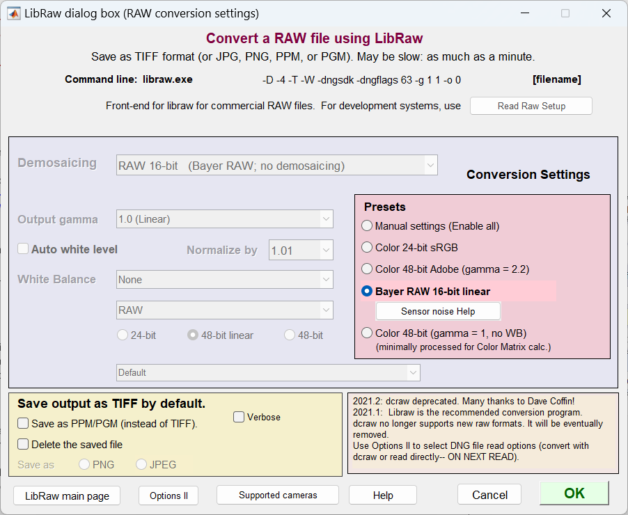 Libraw window (Imatest’s front-end for LibRaw)
An alternative approach to reading commercial raw files, presented in Appendix I. Direct DNG read of commercial raw files, requires an additional step of converting commercial raw files into DNG format, but has the advantage that black level offset is removed and the saturation level is set to the maximum for the file format (2B-1 for bit depth = B, e.g., 65535 for 16-bit files).
Read custom (binary) raw files with Generalized Read Raw
To use Generalized Read RAW, select Settings, Read Raw Setup from the Imatest, Color/Tone Interactive, or Rescharts windows. Enter or select an extension name (3 or 4 characters). “raw” (commonly used but not required) is shown here. Standard RGB file extensions (JPG, PNG, TIF, etc.) and commercial raw file extensions (ARW, NEF, CR2, etc.) should be avoided. The pixel size, width and height settings shown below should be entered for the specific device under test.
You can test the settings by specifying an Output file format and pressing the Convert / Test button on the lower-left. If you make an incorrect choice of sensor pixel size (Width * Height ≠ total pixels in file) the Test function will display the periodicity and suggested values. For RAW noise analysis, set White Balance to None, Demosaicing to none, White level to No change, and Bit shift Pixel offset to 0. Click Save to save the settings or OK to save the settings and close the window.
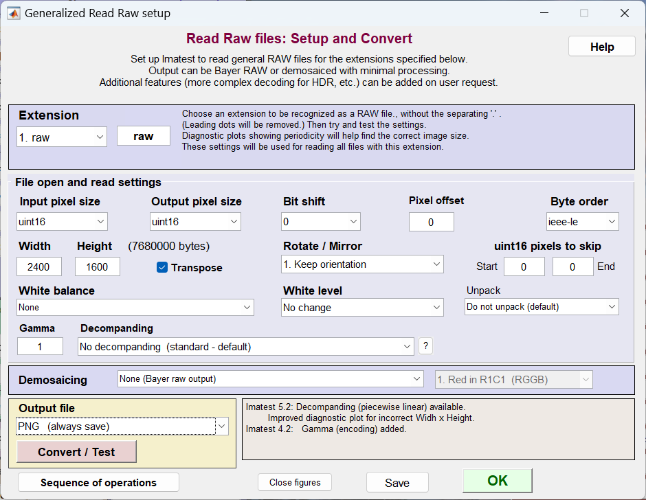 Generalized Read Raw window
Once the settings for the selected file extension has been saved, the image file can be read directly into Color/Tone. Use Convert / Test to convert and save the image (in a standard RGB format) if the ReadRaw window is open.
Process the Bayer Raw image
|
When used with the recommended settings (above), both LibRaw and Generalized Read Raw produce a monochrome image file that contains Bayer RAW image data, defined by a Bayer Color Filter Array (CFA), which covers the pixels in most color image sensors. The CFA makes each pixel sensitive to a single primary color, Red, Green, or Blue. A common order of the colors (“RGGB”) is RGRGRG…, GBGBGB…, etc., in alternating rows. There are twice as many greens as reds or blues because the eye is most sensitive to green. The four possible pixel arrangements (Red locations) are shown on the right, where pixel locations start with Row 1 Column 1 (R1C1) at the upper left corner. There is no universal standard for mapping colors (R, G, or B) to pixel position (RmCn). The arrangement can be determined by examining a Bayer raw image file that contains recognizable colors with the Imatest Rawview utility. |
|
Whenever a monochrome image file is read, the dialog box shown below opens, allowing you to select the image type:
- Standard monochrome,
- Bayer RAW (undemosaiced), or
- Demosaic (convert from Bayer RAW to a full resolution color image using Matlab’s relatively simple but high quality routine).
For measuring image sensor noise, .
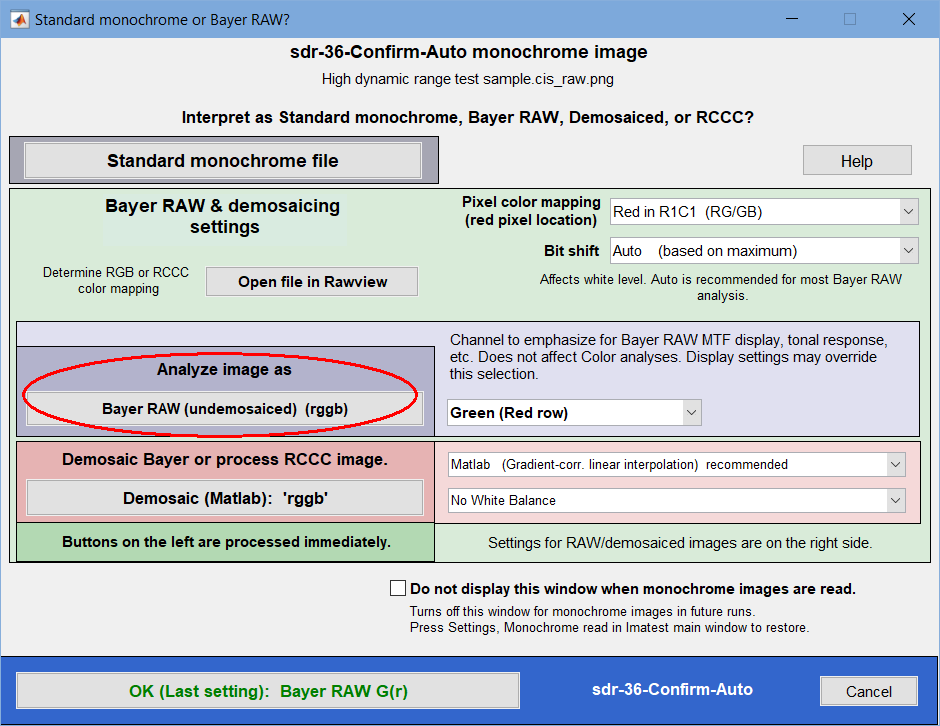 Interpretation of monochrome (or Bayer RAW) file.
Select for analyzing sensor noise.
Black level offset and Saturation level
Most raw images, read from files without demosaicing, are not exactly raw, i.e., their measured Digital Numbers are not identical to the output of the image sensor. The key differences are
- Black level offset DNoff (also called “pedestal” or “DN offset”), added so noise in dark regions does not clip, making it easier to detect dead pixels. Veiling glare (fogging of dark areas caused by stray light) closely resembles black level offset. If not removed, offset results in erroneous estimates of SNR in dark regions as well as dynamic range.
- Saturation (maximum) level, which may be 2N-1 for N-bit analog-to-digital converters (ADCs) or 2B-1 for file formats with bit depth of B. Examples: saturation level = 4095, 16383, or 65535 for N or B = 12, 14, or 16 bits. Or the saturation may be entirely different, i.e., 15070. It must be set correctly to get correct results. Saturation level should not be confused with (well) saturation capacity (usually expressed in electrons, e-), which is a property of the image sensor.
For RGB color files demosaiced with LibRaw, the black level offset is normally removed and the saturation level is set to 2B-1 for bit depth B.
![]() for raw images, Black level offset DNoff and Saturation level should be entered in the Color/Tone Settings window, a portion of which is shown on the right. We recommend starting with a good guess for DNoff, as explained below, then checking Optimize, which uses the algorithm in Appendix 2.1) to obtain the best results.
for raw images, Black level offset DNoff and Saturation level should be entered in the Color/Tone Settings window, a portion of which is shown on the right. We recommend starting with a good guess for DNoff, as explained below, then checking Optimize, which uses the algorithm in Appendix 2.1) to obtain the best results.
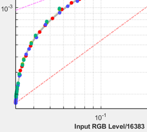
(Initial) black level offset can be estimated by using the following techniques. If it is not removed, the noise levels for the darkest patches tend to be strongly clustered around a level close to the offset in the Photon Transfer Curve, as shown on the right.
- If you are working with a development system and have complete control over the image processing (the ISP), you should know the SN offset.
 Black level offset and Saturation level are often included in the EXIF data in commercial camera raw files (but rarely in JPEG files), but the EXIF data is not entirely reliable: the actual values may be different. The table below contains a few examples from (mostly old) cameras in our lab. The EXIF field names tend to be different for different manufacturers.
 - The offset is smaller than the minimum patch level (which must be ≥ 0 after the offset is removed), but may be larger than the minimum (individual) pixel level. Knowing this, you can apply trial trial-end-error to find the offset. We recommend choosing the largest value that does not cut off the tonal response, but…
Checking the Optimize checkbox, on the right of the DN offset Edit box, improves the estimate of DNoff so the image sensor noise properties can be reliably calculated, as explained in Appendix 2.1.
| Camera – extension / CFA | EXIF data of interest | Values |
| Canon EOS 6D – CR2 [R1C1; RGGB] |
Average Black Level Per Channel Black Level Normal White Level Specular White Level |
2047 (×4) 2047 (×4) 14558 15070 |
|
Nikon D800E – NEF |
Black Level (likely added in the DNG conversion; nothing in the NEF) White Level (also likely added in DNG conv.) [What are WB GRBG levels 256 475 353 256?] |
0 15520 |
| Panasonic FZ1000 – RW2 [R2C1; GBRG] |
Black Level Red, Green, Blue Linearity Limit Red, Green, Blue |
127 4095 |
| Panasonic Lumix G3, LX5 – RW2 [R1C2; GRBG] | Black Level Red, Green, Blue (143 is often observed) Linearity Limit Red, Green, Blue |
128 4095 |
| Panasonic Lumix LX100 [R2C2; BGGR] |
Black Level Red, Green, Blue (143 is often observed) Linearity Limit Red, Green, Blue |
128 4095 |
| Sony A7Rii, A7R5, A6000 – ARW [R1C1; RGGB] |
Black Level White Level |
512 (×4) 15360 (×3) |
Note that different cameras from the same manufacturer may have different Color Filter Array (CFA) configurations.
|
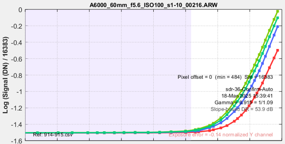
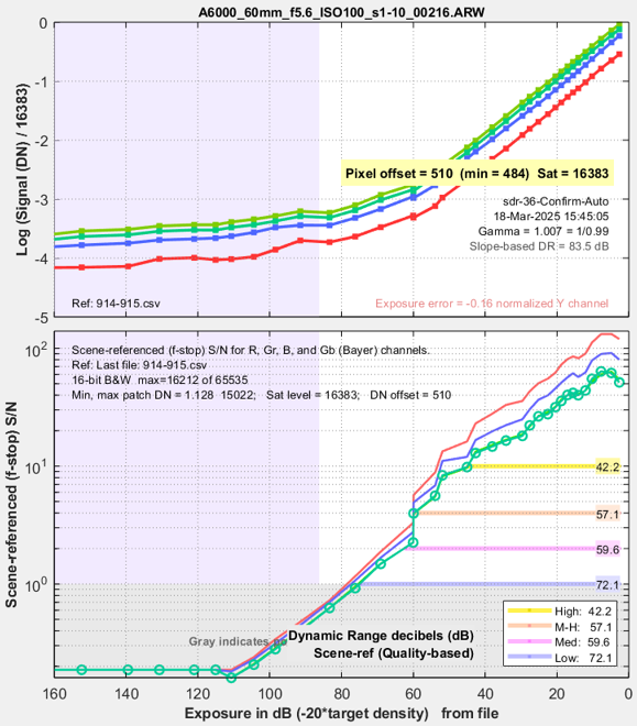
Black level offset DNoff can be recognized as a flattening of the log pixel level response (sometimes difficult to distinguish from flare light). Pixel offsets are sometimes powers of 2 minus 1 (2N-1 = 127, 2047, 16383, …). Most commercial raw files are good examples. When dcraw converts raw files with normal demosaicing, the pixel offset is removed. Images look good and the expected value of gamma is obtained. But when raw files are converted to 16-bit Bayer raw files without demosaicing, the offset is not removed and the saturation level may be lower than the maximum for the file format (e.g., 65535 for bit depth = B = 16). The figures below, from Color/Tone Interactive, show Log pixel vs. log exposure (the tonal response curve) for an undemosaiced image from a Sony micro Four Thirds camera. The minimum pixel level is 488 and the minimum patch level (the mean of the pixels in the darkest patch) is 513, which appears to correspond to a pixel offset of 512 bits. Extreme flattening is visible with no offset correction (on the left). There is still some flattening (likely caused by flare light or dark (Poisson) noise) when the offset is corrected. |
|
Note the y-axis scale: -1.6 – 0. |
Note the y-axis scale: -5 – 0. |
Image sensor noise model — equations
Now — finally — we reach the heart of the calculation: the image sensor noise model.
Although Image sensor noise originates from multiple sources, just three parameters are required for an image sensor performance model.
- Dark noise — noise that appears in the absence of light. Consists of dark current noise, electronic (Johnson) noise, Dark Signal Non-Uniformity (DSNU), and other sources described in OnSemi Application Note AND9189/D..
- Photon shot noise — a Poisson-distributed noise, closely resembling Gaussian noise for more than a mean of 10 electrons per pixel.
- Fixed-pattern noise — caused by random variations of the transistor gain at each pixel. Related to PRNU (Photo Response Non-Uniformity, but not DSNU).
The Digital Number at the image sensor is
DN = DNmeas – DNoff where DNoff is the black level offset, described in detail above.
The normalized signal at the image sensor, used in the equations, is
V = DN / DNmax
where DNmax is the maximum allowable Digital number for the sensor, which is normally 2B-1 for demosaiced RGB signals with bit depth = B (256 for B = 8 or 65535 for B = 16). Programs that demosaic images typically normalize DN to this level, but images processed without demosaicing, so the data is unchanged from raw data, are usually not normalized. For files with bit depth = B = 16 and ADC (Analog-to-Digital Converter) precision a < 16, DNsat is often lower (2a-1 ): 4095 for a = 12 or 16383 for a = 14, although the values may be different. Saturation level is described above.
The noise model used as input to Simatest is derived from two sources: the book, “Photon Transfer DN → λ” by James R. Janesick and the EMVA 1288 standard. The expected (modeled) noise (standard deviation) is
\(\sigma_N = \sqrt{k_{Ndark}^2 + k_{Nshot}^2 V + k_{FPN}^2 V^2}\)
where
σN(V) is the total image sensor noise amplitude (the standard deviation of the noise voltage),
expressed as a function of the normalized signal V. σN2(V) is the variance (or power).
kNdark is the coefficient of the dark noise, or equivalently, the dark noise amplitude. k2Ndark is the dark noise power.
kNshot is the coefficient of the photon shot noise.
kFPN is the coefficient of the Fixed-Pattern Noise (derived from PRNU).
| The key thing to note about this model is that it is based on the Photon Transfer Curve, where noise is a function of the image sensor signal (V = =DN/DNmax), rather than the more familiar Tonal response curve, where signal and noise are functions of exposure (or −chart density). |
The three coefficients are found using a Levenberg-Marquardt optimizer to minimize an array consisting of the differences between the squares of the data points (the R, G, and B circles, below) and the calculated values of σN2(V) (the thick gray curve, below), weighted to emphasize the darker regions so kNdark can be calculated accurately.
|
Using these equations, Imatest can measure sensor noise and dynamic range from unprocessed raw files even if the test chart’s tonal range is less than the sensor’s dynamic range. Although this method provides answers with low tonal range charts such as the X-Rite Colorchecker, we recommend a chart with a large tonal range (usually transmissive), such as one of the Imatest Dynamic Range charts, for best results. |
Run Color/Tone and calculate additional results
The next step is to read a raw image file and look at the results. We choose a raw (ARW) image file from the Sony A6000, a 24 MP Micro Four-Thirds camera with 3.88 μm pixels set to ISO (EI) 100.
Following the steps above, read the ARW file, convert it to Bayer RAW 16-bit linear, select Bayer RAW Red in R1C1 (RGGB.), etc.
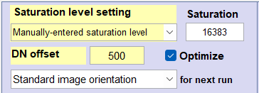
A portion of the settings window is shown on the right. Some of the entries need explanation.
Saturation level setting should be set manually for Bayer raw (undemosaiced) files. The EXIF data for this camera says the maximum value should be 15360, but the largest measured DN is 16148 (as they say, “trust but verify”).16383 was chosen because it is only slightly higher and is 214−1. The ADC is evidently 14 bits.
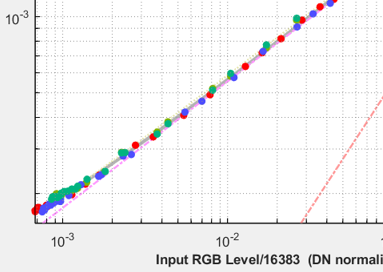
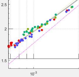
![]() DN (black level) offset is set to an initial value of 510 (the EXIF data indicates 512), and Optimize is checked. Optimize adjusts the offset for plots 10-12 (the Photon Transfer curves) so the ratio of maximum/minimum Digital Numbers, which can be very low when the offset is not subtracted, is increased to 104 or 10(maximum-minimum chart density), whichever is lower. The optimized offset is 511.0. This somewhat kludgy procedure, which only affects the Digital Numbers but not the signal and noise, results in an excellent estimate of the offset, enabling a reliable calculation of the noise coefficients. Without it, data points can be clustered on the left (low DNs; shown for offset = 480 in the thumbnail on the left), making it impossible to reliably calculate the coefficients (especially for dark noise).
DN (black level) offset is set to an initial value of 510 (the EXIF data indicates 512), and Optimize is checked. Optimize adjusts the offset for plots 10-12 (the Photon Transfer curves) so the ratio of maximum/minimum Digital Numbers, which can be very low when the offset is not subtracted, is increased to 104 or 10(maximum-minimum chart density), whichever is lower. The optimized offset is 511.0. This somewhat kludgy procedure, which only affects the Digital Numbers but not the signal and noise, results in an excellent estimate of the offset, enabling a reliable calculation of the noise coefficients. Without it, data points can be clustered on the left (low DNs; shown for offset = 480 in the thumbnail on the left), making it impossible to reliably calculate the coefficients (especially for dark noise).
Here is the result. The Red, Green (two shades), and Blue circles are the original data. the thick gray line is the fit to the σN equation, above. The fit is so good that it’s difficult to see the gray line in parts of the curve.
![]() Photon transfer noise plot (noise vs. normalized input RGB level, adjusted for Black level offset)
Photon transfer noise plot (noise vs. normalized input RGB level, adjusted for Black level offset)
Results to enter into Simatest: kNdark = 0.0001672; kNshot = 0.005554; kFPN = 0.005477; RGB = 0.306, 1.0, 0.606
Saturation capacity in electrons (e-) is derived from the photon shot noise SNR (not the total SNR) in the patch with the highest noise. We call the signal at this patch Vsat to distinguish it from the maximum allowable signal, Vmax. Only the photon shot noise, kNshot2Vsat, is appropriate to use, since it’s the square root of the mean number of electrons. (Note that noise decreases as saturation is approached — it’s zero when the sensor is fully saturated.) The maximum noise is found at Vsat = Normalized DNsat = 0.9169. In this patch,
\(\displaystyle\text{Shot SNR} = \frac{V_{sat}}{ \sigma_{shot}} = \frac{V_{sat}}{ \sqrt{k_{Nshot}^2 V_{sat}}} = \frac{\sqrt{V_{sat}}}{k_{Nshot}} = \frac{\sqrt{0.9169}}{0.005554} = 172.4\).
Saturation capacity is therefore Csat = (Shot SNR)2 = 29724 e- (electrons).
Gain in Digital Number per electron (DN/e-) is derived from Saturation capacity. Recalling that \(V=DN / DN_{max}\),
\(\text{Gain} (DN/e-) = DN_{max} \times V_{sat} / C_{sat} = 16383 \times 0.9169 / 29724 = 0.5054.\)
Noting that \(C_{sat} = (\text{Shot SNR})^2 = V_{sat}^2 / (k_{Nshot}^2 V_{sat}) = V_{sat}/k_{Nshot}^2,\ \text {and hence } V_{sat}/C_{sat} = k_{Nshot}^2\), the equation for Gain (DN/e−) simplifies to
\(\text{Gain} (DN/e-) = DN_{max} \times k_{Nshot}^2 = 16383 \times 0.005554^2 = 0.5054.\)
Since many Imatest results use normalized Digital Number V = DN/DNmax, we sometimes use
\(\text{Gain} (V/e-) = \text{Gain} (DN/e-) / DN_{max} = k^2_{Nshot} = 3.0847 \times 10^{-5}\)
Note that 1/Gain (e-/V) = e- per normalized signal = 32418 is displayed above (with a slight rounding error).
Dynamic Range — sensor and camera
Here is the curve for SNR (dB) for the same image.
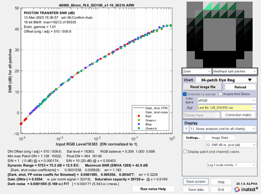 Photon transfer SNR (dB) plot (noise vs. normalized input RGB level, adjusted for Black level offset)
The sensor dynamic range is the difference in densities for the patch with the maximum noise and the patch with SNR = 1 (0 dB). 12.5 EV = 75.2 dB.
The maximum SNR (shown in the Photon transfer SNR (dB) plot, below) is 42.0 dB = 10^(42.0/20) = 125.9.
|
The grayscale tonal response curve (shown on the right) is displayed in several noise plots (but not Photon Transfer plots 10-12). The large offset (about 511 of 4095) has not been removed in the plot on the right. Hence the minimum of log10(signal/16383) is only -1.5. This result is more reliable when black level offset, DNoff , has been removed, as shown on the right, below. |
 |
|
Note that the sensor dynamic range is not the same as the camera dynamic range, which includes the effects of lens flare and is also very sensitive to the experimental setup, where reflected light on the front of the test chart can seriously degrade the measurement. Camera dynamic range for the same image is shown on the right: the ARW raw image was converted to 16 bit linear Bayer raw (uindemosaiced) format with LibRaw. 4 The low-quality dynamic range (72.1 dB), defined by scene-referenced SNR ≥ 1 = 0dB corresponds most closely to the sensor dynamic range (75.2 dB). In this case the numbers are close because we are near the threshold of where flare light from the high quality 60mm prime macro lens (described here) starts limiting the camera dynamic range. Sensor and camera dynamic range diverge when flare light is significant. For reference, ISO 15739 dynamic range for this image is 10 f-stops = 60.2 dB. It was calculated using the patch closest to density = 2.0, even though the chart density goes much higher. This measurement is primarily useful for reflective charts, which rarely go much beyond density = 2.0. |
 |
EMVA 1288
The EMVA (European Machine Vision Association) 1288 standard has a comprehensive set of measurements for image sensor quality that requires capturing multiple dark images and flat field images at half the maximum amplitude. The Imatest Flat Field module has several EMVA calculations, but does not yet measure quantum efficiency and omits some of the measurements needed for a performance model. News: EMVA 1288 will be incorporated into the upcoming ISO 24942 standard.
We recommend the excellent introduction to the EMVA (European Machine Vision Association) 1288 standard. See www.emva.org/standards-technology/emva-1288/ and also www.emva.org/wp-content/uploads/EMVA1288-3.1a.pdf (the standard itself).
The image sensor noise model on this page is a simplified subset of the full EMVA measurements. We can’t claim that it’s EMVA-compliant, but it is EMVA-compatible, so that published EMVA measurements can be used to derive the image sensor noise model.
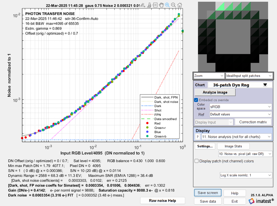
The results below are for a panoramic camera that uses a Sony image sensor. The Photon Transfer Curve below has units of normalized Digital Number, V = DN / DNmax .
![]() Imatest Photon Transfer noise plot for camera with Sony image sensor
Imatest Photon Transfer noise plot for camera with Sony image sensor
| Measurement | EMVA | Imatest |
| Dynamic Range | 69.7 dB | 68.8 dB |
| SNR (Max) | 39.6 dB | 38.4 dB |
| Saturation Capacity in electrons | 9091 e- | 8334 e- |
| Dark Noise σDk | 2.36 e- | N/A |
| Gain (Digital Numbers / electron) | 0.425 DN/e- | 0.41 DN/e- |
| Dark Current, iDark (electrons/second) | 2.22 e- / s | N/A |
| Dark Signal Non-Uniformity, DSNU (electrons) | 0.703 e- | N/A |
| Total Dark Noise = sqrt(σ2Dk + DSNU2 + (iDark × s)2) | 2.43 e- | 3.207 |
| Photo Response Non-Uniformity, PRNU (fraction) | 0.00678 | 0.00499 |
| ADC (Analog-to-Digital Converter: from the spec; not measured) | 12-bit (4095 max) |
Results shown in Boldface can be used to calculate the Photon Transfer Curve coefficients.
The table below shows how to use EMVA 1288 results as input to Simatest and compares original with simulated results. The equations are derived in Appendix 2.3.
| Parameter | Equation: EMVA → Imatest for units of Normalized Digital Number = V = DN / DNmax |
EMVA measured |
Imatest measured |
EMVA simulated* | Imatest simulated* |
| Gain(DN/e−) | Units are Digital Numbers per Electron | 0.425 DN/e- | 0.41 DN/e- | 0.4307 | 0.4142 |
| kNDark | \(\displaystyle \sqrt{\sigma^2_{Dk}+DSNU^2 + (i_{Dark}\ s)^2} \times \text{Gain}(V/e-) \) | 0.0002556 | 0.0003207 | 0.0002772 | 0.0003354 |
| kNshot | \(\displaystyle\ \sqrt{\frac{\text{Gain} (DN/e-)}{DN_{max}}}\) | 0.0102 | 0.01 | 0.001026 | 0.01006 |
| kFPN | \( PRNU(\%)/100 = 0.00687\) | 0.00687 | 0.00499 | 0.006726 | 0.004636 |
| Saturation DN (Maximum) |
Use 2F-1 for F-bit ADCs (Analog-to-Digital Converters) | 4095 | 4095 |
*The last two columns (5 and 6) show that the simulated results from Simatest using the EMVA and Imatest inputs
closely resemble the measured values in columns 3 and 4, as explained in the next section.
Closing the loop
Now we close the loop on the calculations using Imatest results for the Imatest camera and EMVA measurements with the Sony image sensor. We will
- Enter parameters from the above table into Simatest to create test images for two camera models:
- from the Imatest measurements and
- for the EMVA measurements.
- Analyze the images and compare them to the original Imatest results.
Running Simatest
 Open Simatest, then read an image of an ideal 36-patch dynamic range chart. It doesn’t have to be exactly the same as the real physical chart captured in raw format. We use an ideal image, created by the Test Charts module— similar to the images used to create physical test charts. It has a smaller density range than the multi-layer photographic charts.
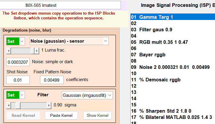
Portions of the Settings window are shown on the right and below. Important settings include
- Noise: simple or dark — kNDark
- Shot Noise — kNshot
- Fixed-Pattern Noise (PRNU) — kFPN
Be sure to press Set with the appropriate line number after entering the values
- Save images — bit depth (16 recommended)
- Offset (DN) — same as the original raw image
- Saturation (DN) — same as the original raw image

Key results are presented in the Summary table, above. Results from the Simatest simulations for the Imatest and EMVA data are extremely close to the results from the original raw images. This shows that Simatest has successfully modeled the image sensor noise. That is what we mean by “closing the loop”.
Here are results of the Simatest model. The x-axis is slightly different from the images above because the simulated chart has a smaller tonal range then the multi-layer photographic UHDR chart.
 Imatest measurements Imatest measurements |
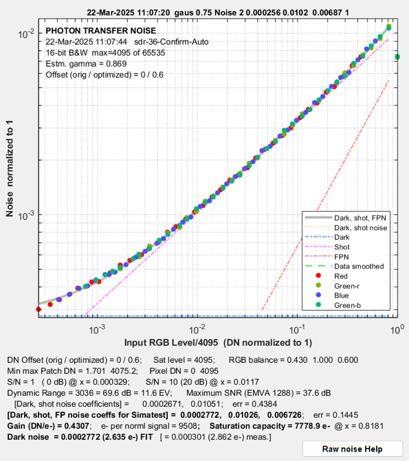 EMVA measurements EMVA measurements |
Results from the Imatest and EMVA measurements are very close, as expected. The Fixed-pattern noise (steep line on the right) is higher for the EMVA measurements, but not high enough to have much effect on the total noise.
Summary
We have presented a sensor noise model that can be used in Simatest simulations to predict the performance of a wide variety of camera systems.
The noise model matches data so well that it’s often difficult to see the thick gray modeled curve behind the input data points.
The model is compatible, though not fully-compliant, with EMVA 1288 measurements. It is much faster and simpler, but somewhat less accurate, and it lacks detail about the two types of fixed-pattern noise (DSNU and PRNU). We show how to use EMVA results, including DSNU and PRNU summary metrics, as input to Simatest.
We are currently using only the EMVA 1288 linear standard. Adding support for the nonlinear standard, which applies to more general sensors, could be challenging.
Right now it does not use photometric measurements (quantum efficiency, etc.). We plan to add results that use EMVA quantum efficiency measurements, and we ultimately plan to add techniques to measure quantum efficiency, which will require specialized hardware. We also plan to support HDR image sensors.
Appendix 1. Direct DNG read of commercial raw files
Issues with the black level offset, DNoff, and saturation white level can be minimized by converting commercial raw files (CR2, NEF, RW2, etc.) to Adobe DNG format, then reading them directly into Imatest— bypassing LibRaw. This description is based on Raw Files— Direct DNG (Adobe Digital Negative) read.
Although direct DNG read offers little advantage for demosaiced files, it has an advantage when using undemosaiced files to measure
- image sensor dynamic range, which requires linear undemosaiced (Bayer) raw file data with pixel levels ranging from 0 for pure black to the maximum for the bit format (typically 65535 for 16-bit depth),
- veiling glare, where a pixel level offset (pedestal) can throw off the measurement, and, of course,
- the image sensor noise model.
It can also be useful for commercial raw file formats not supported by the version LibRaw used by Imatest. (Of course you can download an updated version.)
The problem is that different cameras have different black level offsets (minimum pixel values) and white (saturation) levels, and these values can be difficult to determine because manufacturers record them with different EXIF tags (if at all). These values are normally applied by LibRaw when images are demosaiced, but they are ignored, i.e., the black level offset is not removed and the saturation level may unchanged, when images are not demosaiced.
 The black level offset needs to be removed and the saturation level needs to be known for image sensor noise models and dynamic range calculations. This is done automatically when raw files converted to DNG is read directly into Imatest. See Processing Raw Images in MATLAB for an overview.
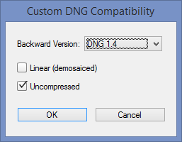
Any commercial raw file (CR2, RW2, NEF, etc.) can be converted to DNG format using Adobe’s free DNG Converter . Download here and follow the instructions. Adobe Digital Negative Converter runs in a GUI window. To use it for undemosaiced files, open it and click Change preferences to open the Preference window, then select Custom… in the Compatibility dropdown window to open the Custom DNG Compatibility window. Linear (demosaiced) should be unchecked and Uncompressed should be checked, as shown on the right.
Operation of the DNG converter is straightforward. Note that all files in a folder will be converted, so if you want only a limited number of files to be converted, you’ll need to move them to a separate folder.
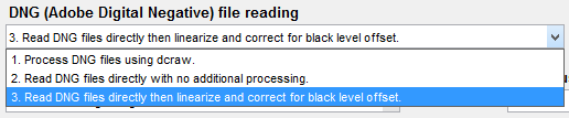 To take advantage of this capability, the setting shown on the right, 3. Read DNG files directly then linearize and correct for black level offset, must be selected in the Options II window, which can be opened from a button on the lower-right of the Imatest main window or in the Settings dropdown menu of the Imatest main or Color/Tone Interactive window. When this setting is selected, DNG files read into Imatest have pixel level = 0 for pure black and have a maximum pixel level of 2bit depth-1: (65535 for bit depth = 16), making them well-suited for measuring sensor dynamic range.
When Direct DNG read has been used, issues involving Black level offset and white level saturation can generally be ignored.
Appendix 2. Algorithms
2.1 Black Level Offset Optimization
The Black Level Offset DNoff must be removed in order to obtain a good distribution of signal and noise levels so the coefficients for dark, shot, and fixed-pattern noise, Ndark , kNshot , and kFPN , can be correctly calculated. Here is an example of Photon Transfer Curves (noise as a function of normalized Digital Number) without and with DNoff removed.
 DNoff not removed |
 DNoff (guess 500) partially removed |
 Offset (DNoff = 511) completely removed |
Here are some subtle but important points about Photon Transfer Curves and Black Level offset.
 The offset does not affect the noise measurement. It is the same in the three plots above, which have different amounts of offset removed. But Signal-to-Noise Ratio (SNR), and hence dynamic range, is affected by the offset.
- The primary benefit of removing the offset is that it allows the noise coefficients, primarily the dark noise coefficient kNdark (which is equal to the dark noise amplitude) to be calculated. Referring to the above images, when the offset is not removed or partially removed, data points are clustered around the minimum signal level (the x-axis), which is approximately, but not exactly, equal to the offset. The image on the right– which is an enlarged portion of the middle image, above, illustrates this clustering. Only when there is some “breathing room” for the low noise values (as in the right image, above), can the three coefficients be separated and calculated correctly.
- An accurate value of DNoff is required to obtain an accurate value of dark noise, kNdark , which is a key performance indicator for image sensors. The shot and fixed-pattern noise coefficients are less sensitive to the estimate of DNoff.
Black level offset DNoff should be set to an initial value, where DNoff is smaller than the minimum patch level (which must be ≥ 0 after the offset is removed), but may be larger than the minimum (individual) pixel level.
Check Optimize in the Setting windows to turn on the optimizer for automatically determining the offset to a value that gives reliable values of the noise coefficients. The optimizer is only applied to the Photon Transfer noise or SNR curves in plots 10-12.
Most plots, except for the Photon transfer plots (10-12), display signal or noise as a function of exposure (-density), i.e., (−)density on the independent (x) axis. The optimizer works with photon transfer curves where noise is a function of the signal, typically expressed in Digital Numbers (DN). The black level offset DNoff adds a fixed value to the signal, which reduces the ratio between the maximum and minimum signals. This causes noise data for the darker patches to be strongly clustered around the minimum level (which includes the offset).
Black level optimization algorithm
The ratio of the measured digital numbers prior to removing the offset is RDN = DNmax/DNmin.
For maximum-minimum chart density = Δden = denmax– denmin , the density ratio is Rden = 10Δden.
The goal of the optimizer is to make the optimized DN ratio,
ROpt = (DNmax − DNoff )/ (DNmin − DNoff ),
large enough so that the dark noise coefficient can be calculated reliably.
We do this by finding the value of DNoff that makes ROpt = min(105, Δden) . The choice of 105 is somewhat arbitrary, determined by trial-and-error. It is larger than we see in real cameras (with veiling glare from lenses). 103 wasn’t large enough to give a reliable result; 104 or 105 work well, but anything greater than 105 is not needed and doesn’t correspond to reality.
ROpt (DNmin − DNoff ) = DNmax − DNoff ; DNoff (1-ROpt ) = DNmax − ROpt DNmin
DNoff = (DNmax − ROpt DNmin) / (1-ROpt )
For the UHDR chart reference file used is several examples , above, Δden = 8.833-0.133 = 8.70. Therefore Rden = 108.70, and ROpt = 105.
2.2 Noise coefficients — initial values and optimization
As we indicated in Image sensor noise model — equations, the expected (modeled) total noise is
\(\sigma_N = \sqrt{k_{Ndark}^2 + k_{Nshot}^2 V + k_{FPN}^2 V^2}\)
where V = DN / DNmax is the normalized signal at the image sensor and DNmax is the maximum allowed Digital number, sometimes equivalent to the saturation Digital Number, DNsat.
The noise coefficients, Ndark, kNshot, and kFPN are the key parameters for the image sensor noise model in the ISP/Camera Simulator program, Simatest. They are found using a Levenberg-Marquardt optimizer that minimizes (σN(n) – σmeas(n))2) for grayscale patches n = {1, …, N}. The patches have normalized digital numbers V(n).
Good initial values of the coefficients are required for the optimizer to give reliable and consistent results.
Sort the N patches from darkest (1) to lightest (N). The measured noise in patch n, where n = {1, …, N} is σmeas(n).
Assume that the initial value of the dark noise coefficient is kNdarkInit = σmeas(1) and the fixed-pattern noise coefficient is kNshotInit = 0. Then since \(\sigma_{N(init)} = \sqrt{k_{NdarkInit}^2 + k_{NshotIinit}^2 V}\),
σmeas(N)2 – σmeas(1)2 = (σmeas(1)2 + kNshotInit2 V(N)) – (σmeas(1)2 + kNshotInit2 V(1))
= kNshotInit2 (V(N) – V(1)) , so that
\(\displaystyle k_{NshotInit} = \sqrt{ \frac{\sigma_{N2}^2 – \sigma_{N1}^2}{V(N) – V(1)}}\)
The optimizer is run twice: first for the full set of coefficients, Ndark , kNshot , and kFPN , and second for a reduced set, Ndark and kNshot (omitting kFPN ). If kFPN < 0 in the first optimization, then the results of the second optimization, which assumes kFPN = 0 , is used.
We tried using the optimizer find DNoff . but It failed because it was not possible to separate its effects from Ndark . Ultimately we settled on the method in 2.1 for finding DNoff , which needs to be removed before calculating the coefficients.
2.3 EMVA 1288 results for Simatest input
EMVA 1288 results shown in the first table in the EMVA 1288 section can be converted into Photon Transfer curve noise coefficients for input to Simatest.
The maximum Digital Number, DNmax, for an image sensor is 2(ADC Precision)-1 = 212-1 = 4095. (This is a specification, rather than an EMVA result.)
The equation for Gain(DN/e−) from the Run Color/Tone section, above, is derived from Saturation capacity. Recalling that \(V=DN / DN_{max}\),
\(\text{Gain} (DN/e-) = DN_{max} \times V_{sat} / C_{sat} = 16383 \times 0.9169 / 29724 = 0.5054.\)
Noting that \(C_{sat} = (\text{Shot SNR})^2 = V_{sat}^2 / (k_{Nshot}^2 V_{sat}) = V_{sat}/k_{Nshot}^2,\ \text {and hence } V_{sat}/C_{sat} = k_{Nsat}^2\), the equation for Gain (DN/e−) simplifies to
\(\text{Gain} (DN/e-) = DN_{max} \times k_{Nsat}^2 = 16383 \times 0.005554^2 = 0.5054.\)
The shot noise coefficient is
\(\displaystyle k_{Nshot} = \sqrt{\frac{\text{Gain} (DN/e-)}{DN_{max}}} = \sqrt{0.425/4095} = 0.0102\)
For dark noise, we need Gain(V/e-) = Gain (DN/e-)/DNmax = 0.425/4095 = 0.0001038. For short exposures, < 0.1s, which would apply to any video camera, it is usually safe to omit the iDark term.
\(\displaystyle k_{Ndark} = \sqrt{\sigma^2_{TmpDk}+DSNU^2 + (i_{Dark} s)^2} \times \text{Gain}(V/e-) \\\qquad= \sqrt{2.36^2+0.703^2} \times 0.0001038 =2.462 \times 0.0001038 = 0.0002556 \)
Finally, the fixed-pattern noise is
\(\displaystyle k_{FPN} = PRNU(\%)/100 = 0.00687\)
2.4 Temporal, Fixed-Pattern, and Total noise
Temporal noise is noise that varies randomly from image to image, in distinction to Fixed-Pattern Noise (FPN), which is constant — the same for each image acquisition.
The method presented here provides less detail about Fixed Pattern Noise than EMVA 1288 and IEEE P2020, both of which require two groups of multiple images (≥30):
- one for dark noise (DSNU = Dark Signal Nonuniformity), and
- one taken at about half saturation (DN ≅ DNmax/2) (PRNU = Photo Response Nonuniformity).
Acquiring multiple images allows FPN to be fully characterized and completely distinguished from temporal noise. FPN is actually an image of sorts — It’s not gaussian; it tends to resemble woven fabric, which is why row and column FPN are often measured. FPN is important for image sensor designers, but it’s less important for measuring image sensor performance, where it causes performance degradation similar to temporal noise (unless it’s compensated, which requires custom calibration for each sensor).
Even though the Imatest image sensor noise model is typically measured with a single image (though a second image can be useful for obtaining dark noise), we can partially separate temporal from Fixed-Pattern Noise because the noise model is derived from three coefficients, each representing a distinct type of noise.
- Dark noise kNdark — combines DSNU (dark signal nonuniformity, i.e., fixed pattern noise), electronic noise (temporal), dark current noise (temporal), and noise from other sources. We cannot separate DSNU fixed pattern noise from other dark noise sources with a single image: At the very minimum, this involves subtracting two identical images. Fortunately DSNU does not have a strong effect on most images, which are Photon Shot noise-dominant.
- Photon Shot noise kNshotV1/2 — increases with the square root of the signal amplitude. It is entirely temporal.
- PRNU Fixed pattern noise kFPNV — increases linearly with the signal amplitude.
As we have noted above, the total noise, which includes temporal and Fixed Pattern Noise is
\(\sigma_{N-total} = \sqrt{k_{Ndark}^2 + k_{Nshot}^2 V + k_{FPN}^2 V^2}\)
For regions where photon shot noise is significantly greater than dark noise, i.e., \(k_{Ndark} « k_{Nshot} \sqrt{V}\),
\(\sigma_{N-temporal} = \sqrt{k_{Ndark}^2 + k_{Nshot}^2 V }\) (omitting k2FPN V2) is a very close approximation to the temporal noise.