Simatest Overview — focusing on what you can do with Simatest
Details on how to use Simatest are in the links below.
|
Simatest ISP/Camera Simulator — Instructions and Reference – Very detailed Simatest examples – Examples of how Simatest can be used. Compares simulations to measurement. Image Sensor Noise – measurement and modeling – using raw files for image sensor Dynamic Range and Simatest Using Color/Tone Interactive – Interactive analysis of color & grayscale test charts Color/Tone & eSFR ISO noise measurements – describes how to measure image sensor noise from raw images Image information metrics – new measurements, based on Shannon information theory, that are superior predictors of Machine Vision system performance |
Demonstration – Introduction – Block diagram – Input images – Recommended test charts
Running Simatest – Settings – Image processing blocks – Processing – Results – Side-by-side view
Controls on the bottom – Analysis and view controls – MTF example – Dropdown menus
Benefits of Simatest – Low Light analysis – Appendix: Image sensor noise model
Simatest is part of Imatest 25.1
Introduction
Simatest — Imatest’s Camera and ISP (Image Signal Processing) Simulator, introduced in early 2025, simulates complete camera systems, including the effects of lens degradations, image sensor noise, and ISP pipelines, enabling all important image quality factors (KPIs) to be predicted. It includes a large set of ISP processing blocks that can be applied in arbitrary order.
Demonstration
| Simatest lets you create software prototypes for – speeding up the development of camera systems and image processing pipelines, and – exploring how lenses, image sensors, and image processing affect camera system performance. |
Input to Simatest consists of
- images — from cameras or simulated, described below,
- physical properties of the camera system including lens blur, image sensor noise, and color balance (a function of illumination and sensor/CFA spectral response). They should not be changed when simulating a specific camera, but they can be adjusted to explore “what-if?” scenarios,
|
Image sensor noise is perhaps the most important camera physical property. Simatest’s image sensor noise model is based on measurements of raw images of grayscale dynamic range charts analyzed by Color/Tone or on EMVA 1288 results. It is highly accurate, and it enables image system performance to be calculated for a wide range ISP design and environments, including low illumination. Since performance is derived from the sensor and noise signal measured in electrons, radiometric measurements (the precise light energy incident on the sensor) are not required, though we plan to add them as options in the near future. This simplifies Simatest operation. The image sensor noise model is summarized in an Appendix at the bottom of this page and in a more detailed description in Image Sensor Noise — Measurement and Modeling. |
We will highlight the (relatively few) physical properties, which can be set along with ISP adjustments in the Settings window.
- adjustments, primarily Image Signal Processing (ISP) that can be made freely.
Simatest block diagram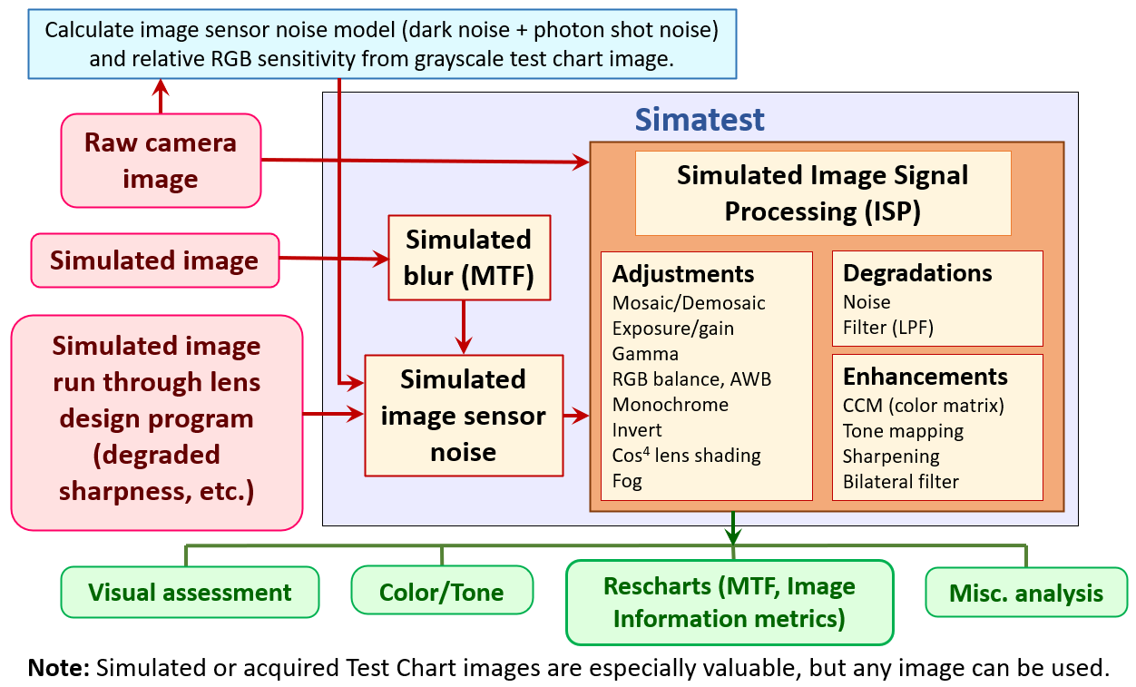
- Raw or minimally-processed camera images acquired from cameras without or with demosaicing, with minimal processing (best with no sharpening, noise reduction, etc.).
- Raw images are used to measure the image sensor noise, as well as RGB color imbalance.
- Minimally-processed demosaiced images are used to estimate lens blur by matching measured MTF with Simatest gaussian-filtered results.
- Highly processed images (found in most consumer camera JPEGs) are not recommended for Simatest input.
- Simulated bitmap test chart images produced by the Imatest Test Charts module,
- Simulated bitmap image files that have been processed to include lens degradations by lens design programs such as Code V or Zemax OpticStudio — recommended if they are available.
Although Simatest can process any pictorial image, test chart images are recommended where quantitative results (MTF, tonal response, information capacity, etc.) are needed. Recommended test chart images are listed below.
Simatest adjustments (processing) include
- Camera and lens image degradations (physical properties of the imaging system), such as noise, fog (veiling glare), and blur, Lens degradations can be modeled as gaussian blur, which is highly simplified, but sufficient for designing and testing ISP.
- Image adjustments, such as exposure (and gain to simulate changing the Exposure Index), gamma, and Bayer demosaicing/mosaicing,
- image enhancements, such as applying a Color Correction Matrix, tone mapping (used in High Dynamic Range (HDR) imaging), Sharpening (two varieties), and bilateral filtering,
- ability to simulate motion blur, misfocus, low light conditions, and more.
Simatest results
- for human vision — results can be immediately viewed in the Simatest interactive window. You can view input and output images individually or side-by-side, enlarged if needed,
- for machine vision — results of processing can be viewed in Simatest, saved in files, or immediately opened in Imatest modules to obtain all major image quality measurements.
- Rescharts: MTF, noise, and image information metrics (information capacity, PSD, NEQ, SNRi, and Edge location σ),
- Color/Tone: Tonal response, noise, SNR, and Photon Transfer Curves, which are used for the image sensor noise model,
- Image Statistics: Spectra, histograms, etc.,
- Miscellaneous results, directly viewable in Simatest, including SSIM, PSNR, MTF (for output/input), Optical Character Recognition (OCR), and Face or People Detection.
Simatest is expandable. Processing blocks will be added as needed, based on customer requests. The initial set of blocks is primarily focused on operations that affect visible and measurable image quality.
Simatest can operate on batches of images, automatically reading, processing and saving images in the batch.
Simatest input images
Simatest input can come from any image file, raw or demosaiced, that is readable by Imatest and listed in Image file formats and acquisition devices. Although Simatest can work with any image, test chart images produce the most useful quantitative results (recommended images are listed here). There are two major sources of input files.
- Ideal test chart images are the input for complete camera system simulations, which may or may not be degraded by passing them through lens design programs.
- Raw or minimally-processed images (without or with demosaicing) are not used for complete camera system simulations, but they have two essential functions.
- They may be images that need to be tuned using the many Image Signal Processing (ISP) blocks.
- As we have noted, they are useful for measuring a camera’s physical properties (image sensor noise, etc.).
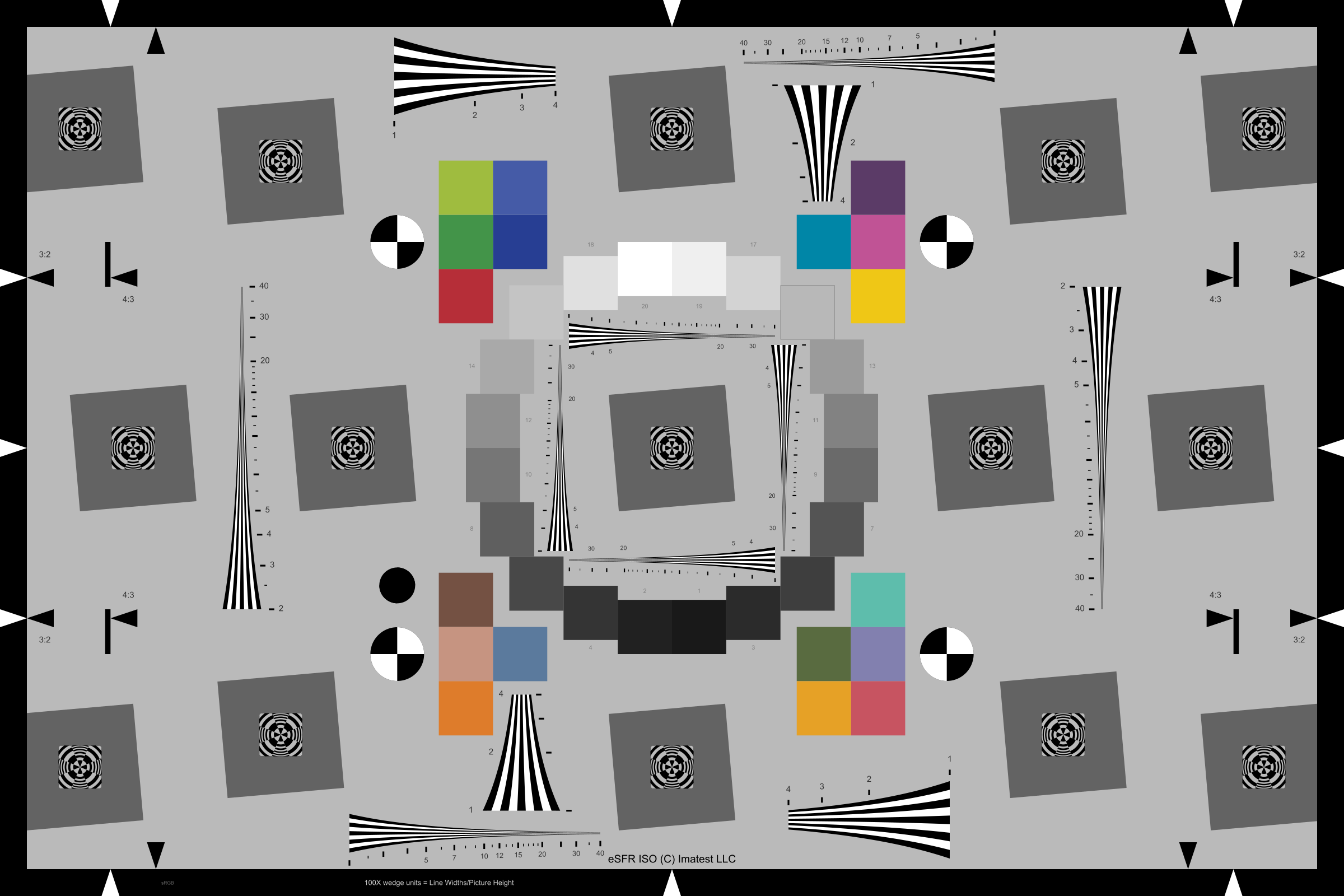
Test Charts program — The most convenient source of ideal test chart images is the Imatest Test Charts program. Here is an example, illustrating settings for creating a 2400×1600 pixel Enhanced eSFR ISO 2017 chart.
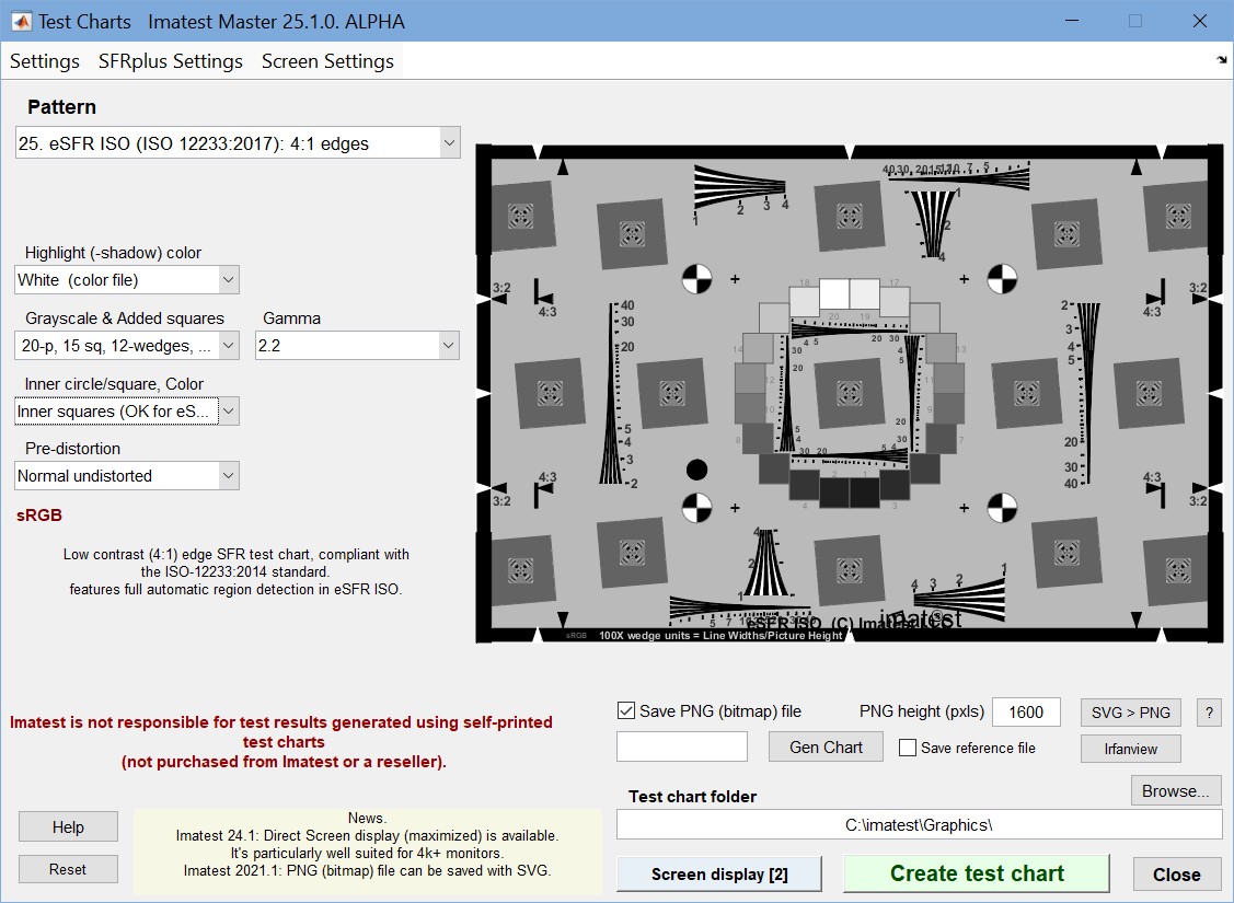 Test Charts window for the Enhanced eSFR ISO 2017 chart
Brief instructions for making Test Charts images are in SImatest – Instructions and Reference. The full documentation is on Test Charts and SVG Test charts. You can also download the 2400×1600 eSFR ISO PNG image (with added color patches) that was used for developing and testing Simatest.
Test Charts lets you create SVG (Scalable Vector Graphics) or bitmap (TIFF or PNG) chart files that can be used for printing physical charts or for analyzing chart images. It supports a great many chart types and options. eSFR ISO (ISO 12233-2014 or 2017) and 36-patch dynamic range charts are created as SVG files, which can be opened by Inkscape (an excellent free program) for conversion to 16 or 48-bit PNG or TIFF bitmap files (strongly recommended, especially for tonal response measurements).
Images intended for viewing or printing should be created with Gamma = 2.2 (the display or color space gamma). When using these images in Simatest, set Input gamma = 0.45. Images intended for degradation with lens design programs should be created with gamma = 1 (linear gamma), as described below.
Some Test Charts settings are hidden in dropdown menus. We recommend selecting eSFR LogWedge max = 4000 LW/PH in the Settings dropdown menu.
When your settings are complete, press Create Test Chart , and save the files (you’ll get both SVG and 8/24-bit PNG) in a convenient location.
Lens design programs — such as Code V or Zemax OpticStudio let you process chart images, degrading them (adding blur, chromatic aberration, vignetting, and stray light) using a realistic lens model. The chart images can be created with the Imatest Target Generator, which is a back-end (postprocessor) for Test Charts, converting SVG charts to bitmap files. [This must be verified: Charts for input to Code V must have gamma = 1 (linear gamma). When using these images in Simatest, set Input gamma = 1.] When a lens design program has been used, the Simatest (blur) filter isn’t needed, unless you need to simulate an anti-aliasing (optical lowpass) filter.
Images acquired from cameras — Raw or minimally-processed images, converted to RGB with LibRaw or ReadRaw, work well. These include the actual images from development systems that need to be tuned. Blur and noise are already present in these images, so (blur) Filter and Noise blocks won’t be needed.
Most JPEG images from consumer cameras should be avoided because they are heavily processed, including complex tonal response curves (with “shoulders”) and nonlinear and nonuniform bilateral filtering, making it difficult to obtain useful results.
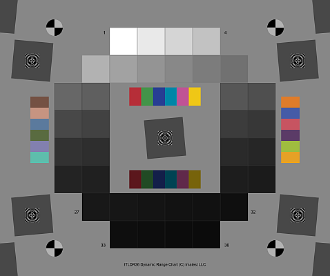
Recommended test charts
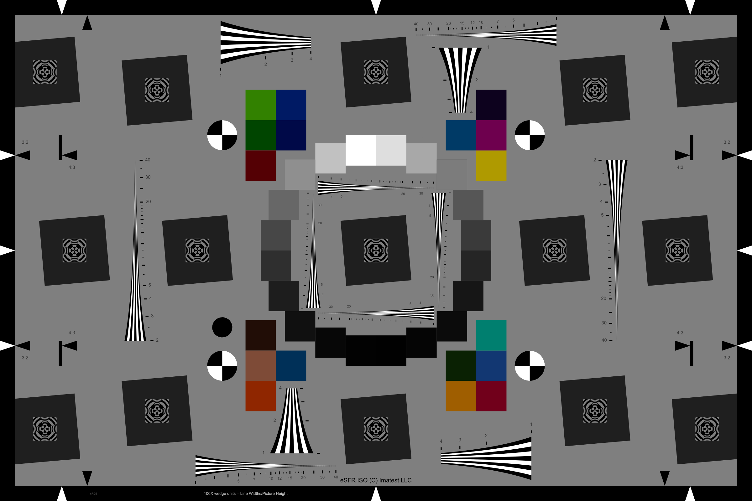
36-patch charts are particularly valuable for measuring image sensor noise (Photon Transfer Curves). They were used for simulations in Simatest Overview, Simatest Examples and Image Sensor Noise — measurement and modeling. Simulated results correlate well with physical measurements because Photon Transfer Curves, MTF, and color measurements are relatively insensitive to region size. The total image size can be different in the simulated and measured images; they do not need to fill the frame, especially for high resolution images where barrel distortion (from fisheye lenses) or light falloff (vignetting) may be issues. You can download a 48-bit color 1901×1600 version of the image here. For images degraded by lens design programs — We recommend eSFR ISO charts (either the enhanced (3:2) or extended (16:9) versions), which are designed to fill the frame and should have the same size (in pixels) as the image sensor. We include SVG files for two eSFR ISO charts that should work for most applications. They can be converted to bitmap files in Inkscape, and they can be cropped or padded as needed. Note that they look dark because they were created with gamma = 1. Zip file with all Simatest SVG & PNG test chart images | Enhanced eSFR ISO PNG | Extended eSFR ISO PNG |
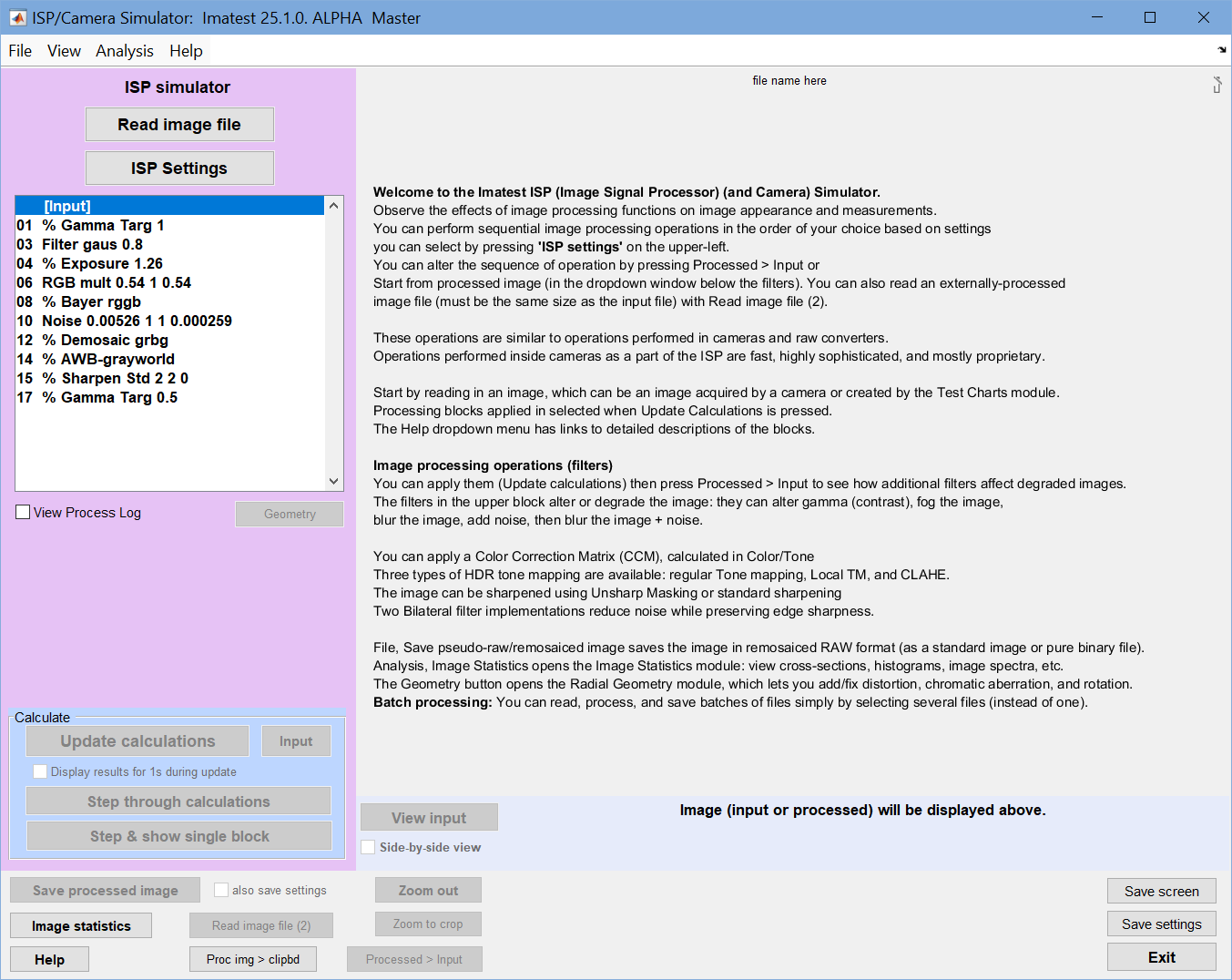
Simatest opening window
Running Simatest
Press Simatest in the the Utility dropdown menu or in the Utility tab on the right of the Imatest main window. To perform an analysis,
- Read an image file, Batch (multiple) files are supported.
- Open the Simatest Settings window, described below, if needed. Settings are saved from the previous run.
- Update the calculations. They will be updated automatically if Auto update in the lower-right of the settings window is checked.
- Display results of interest, either visually in Simatest, or by directly opening the processed image directly to Rescharts, Color/Tone, or Image Statistics.
The order of pressing Read image file and Simatest Settings is unimportant.
Here is the Simatest window after updating. In this case the processed image, shown unenlarged, is quite close to the input image. The input and output images can look very different when enlarged and viewed side-by-side, as shown below.
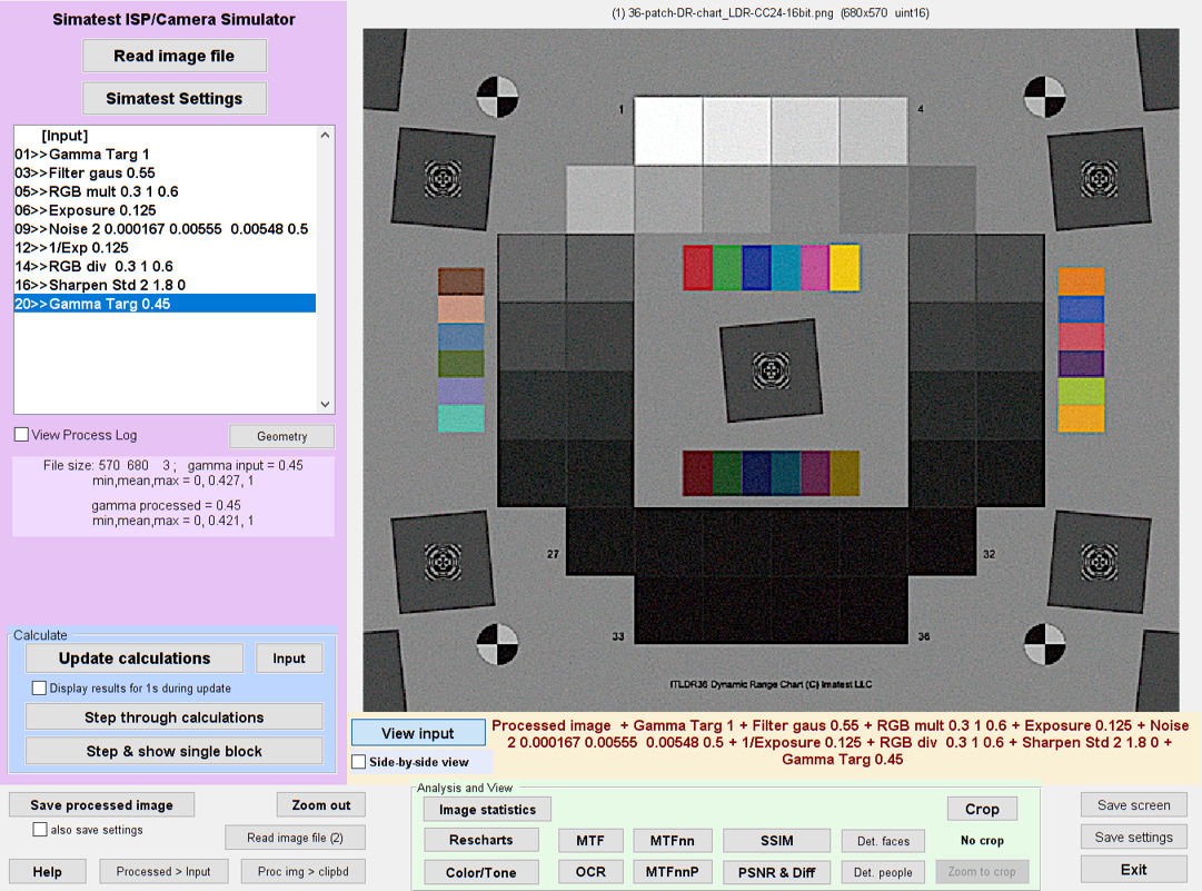
Simatest window showing processed image (View input for input image)
The Simatest Settings window lets you set up the analysis: you can select processing blocks, and adjust their parameters and set the order of operations.
The Settings window contains a large number of processing blocks. Some, like Sharpen, Tone mapping, or Bilateral Filter, have several methods (algorithms) and associated parameters and are contained inside rectangular frames.
The Simatest settings are divided into five regions: 1. Input processing & degradations, 2. Degradations (noise, blur), 3. Color and tone adjustments, 4. Sharpening/noise reduction, and 5. Image file save settings. Some categories overlap, e.g., since cos4 lens shading either adds and corrects for vignetting, we put it in Adjustments rather than Degradations.
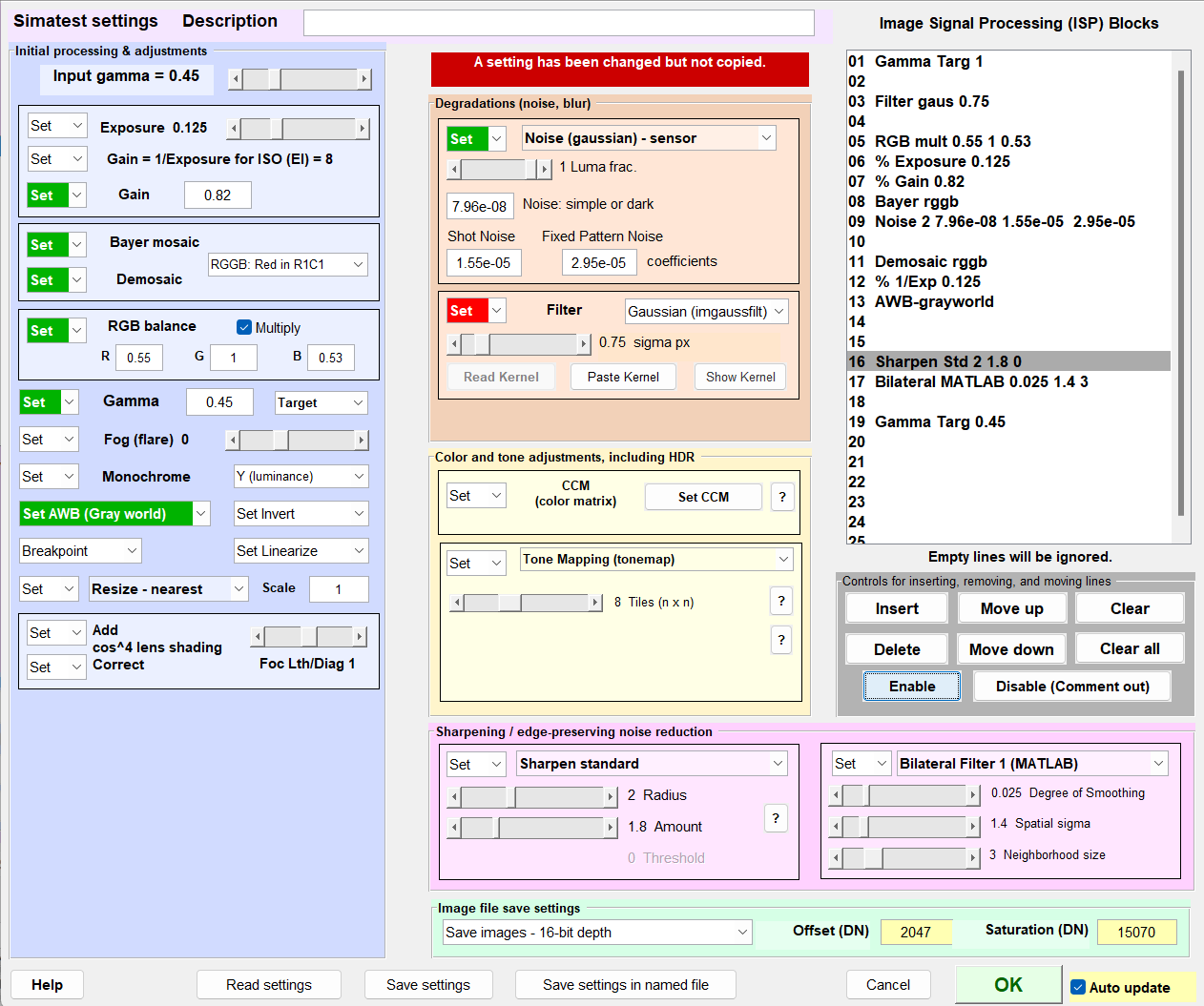 Simatest settings window
The Image Signal Processing (ISP) Blocks box, on the upper-right, contains the sequence of operations. Blank lines are intended to make it easy to insert, arrange, and delete entries, and are ignored when the settings are transferred to the main window or processed.
SUMMARY: Settings are made in two steps: Since it’s easy to forget the Step (2), Set dropdowns are changed to White with a red background when the corresponding parameter has been adjusted, but not yet moved. |
Image processing blocks
Depending on the input image source, some degradations or enhancements may have been performed in the camera prior to entering the image into Simatest. For example, JPEGs from consumer cameras (not recommended for Simatest input) typically have nonlinear, nonuniform bilateral filtering. For camera images, you don’t need to add noise or blur filtering because they have already been implicitly applied.
| Quick links to physical properties of camera systems, which are highlighed below. Other blocks are image signal processing (ISP). RGB Balance – Multiply – Fog – Image sensor noise |
| Processing block | Description | Function link |
|
| Input gamma | Required for keeping track of the image gamma at each state of the processing — important because some operations require the image to be linear (gamma = 1). | Gamma, Tonal Response Curves | |
| Initial processing & adjustments | |||
| Exposure Gain = 1/Exposure Gain (set by slider) |
Exposure/gain multiplier or divider (gamma = 1 (linear) required) lets you attenuate or boost the signal.
|
(L) |
|
| Demosaic Bayer mosaic |
Demosaic converts a Color Filter Array (CFA)-mosaiced Bayer raw image from an image sensor (monochrome format) into a 3-color RGB file using the MATLAB demosaic function, which has some weaknesses (“zippering” between boundaries of different colors). Bayer mosaic (the inverse of Demosaic) converts 3-color RGB images into monochrome, mosaiced, pseudo-raw images. |
demosaic Imatest raw processing | |
| RGB Balance — Multiply or Divide ( a camera physical property ) |
RGB Balance — Multiply simulates RGB imbalance, which is displayed in noise plots 10-12 (Photon Transfer Curves) from raw images — illustrated in the same image used to measure image sensor noise. RGB Balance – Divide is the inverse of Multiply: corrects the imbalance. |
(L) | |
| Fog (flare or veiling glare) ( a camera physical property ) | Add a constant value to fog the image — equivalent to adding flare light or veiling glare. Negative values can be used to remove black level offset, if present. |
|
|
| Monochrome | Convert (m×n×3) color images into monochrome (m×n) using either a luminance equation or mean. | ||
| AWB (Auto White Balance) | Perform Auto White Balance using the simple “gray world” algorithm. |
|
|
| Linearize (Set) | Linearize the image (equivalent to Gamma target 1). Required or recommended for most ISP blocks. | ||
| Gamma | Adjust the gamma encoding of an image. Selected by an edit box and a popup menu that contains Target and Mult for target gamma or gamma multiplier. Important because color space files are usually gamma-encoded (often with gamma ≅ 0.45), but many operations require gamma = 1. | Gamma, Tonal Response Curves | |
| Add, correct cos4 lens shading | Add or correct vignetting (light falloff) using the standard cos4 angular equation. Lens focal length/sensor diagonal distance must be entered using the slider. Appropriate for simulated images early in the ISP pipeline, before noise has been added.Already present in real camera images. | (L) | |
| Invert (Set) | Invert the image, i.e., turn it into a negative. Infrequently used. | ||
| Resize | Resize the image by multiplying size by Scale. Three methods are available. | ||
| Image degradations: blur, noise, geometry Often found in images acquired from cameras prior to processing. Operations are generally linear. |
|||
|
Noise (Gaussian) ( a camera physical property ) |
Add noise to the image. Key selections: Noise (gaussian) – simple: Simple, signal-independent noise. Noise (gaussian) – sensor: Signal-dependent image sensor noise, described below and in Image Sensor Noise. These include dark, photon shot, and fixed-pattern (PRNU) noise. Present in all physical image sensors. |
||
| Filter ( a camera physical property ) |
Filter (blur) the image. Typically applied before noise. Options: Gaussian, Mortion blur, Disk (for mosfocus), Airy disk (for diffraction), or arbitrary kernel. A gaussian filter can be used to simulate lens blur (in one region). |
imgaussfilt filter2, imfilter Simple Airy pattern |
|
| Radial Geometry | Add or correct optical distortion (using any of several models) and/or Lateral Chromatic Aberration. | Radial Geometry | |
| Tonal enhancement: Correct colors or apply one of three tone mapping algorithms, | |||
| Color Correction Matrix (CCM) | Apply a Color Correction Matrix (CCM), which can be calculated and saved in Color/Tone. As of March 2025, not yet well-integrated into Simatest: The CCM must be calculated before running Simatest. | Color Correction Matrix, calculated in Color/Tone. | |
| Note that there are three tone mapping blocks: same purpose but different algorithms. | |||
| Tone mapping (three types) |
Render high dynamic range (HDR) image for viewing in displays with limited dynamic range. Nonuniform and nonlinear Three types are available. tonemap: Render high dynamic range image for viewing localtonemap: Local tone mapping Contrast-Limited Adaptive Histogram Equalization (CLAHE) adapthisteq |
||
| Spatial enhancement: sharpening and/or noise reduction. |
|||
| Sharpen USM or Standard | Sharpens the input image using Unsharp masking (USM) or Standard sharpening. which uses a 2D version of the 1D sharpening method described in the Sharpening page. Most visible on edges. | imsharpen: Unsharp Masking (USM) | |
| Bilateral filters (three types)
|
Bilateral filtering, proposed by Tomasi and Manduchi in 1998, is a method for edge-preserving smoothing that keeps edges sharp while smoothing other areas. Widely used in consumer JPEG images. Simatest has three implementations. Nonuniform and nonlinear. imbilatfilt (MATLAB) – bfilt2 (Lanman) (slow) – Non-Local Means filter (also slow) |
imbilatfilt (MATLAB) bfilter2 (from the Mathworks File Exchan imnlmfilt (MATLAB) |
|
| Image file save settings: applied when an image is saved in a file. | |||
| Save file Precision | 4. 16-bit, full amplitude, except raw. RGB files have the full amplitude of the container (e.g., 65535 for bit depth = 16) and no offset is recommended. | ||
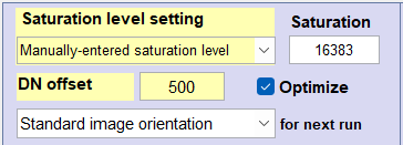
| Save file Offset (DN) | Black Level Offset in pixels (Digital numbers) to be added to saved raw files. Set to duplicate cameras. | ||
| Save file Saturation (DN) |
Saturation Level (maximum pixel or DN level) for the saved file. Used to represent m bit data in an n bit container (e.g., 4095 for m = 12-bit data stored in an n = 16-bit file, where the maximum DN is 65535. | ||
Process the image
- by clicking OK in the Settings window, with Auto update (lower-right checked), or
- using Update calculations or another of of the buttons in the Calculation group (the light blue box on the left of the Simatest window).
| Update calculations | Starting with the input image, process each block shown in the List box. Display the results when processing is complete. This is the most common calculation. |
| Input | Restore the input image view. |
| Display results for 1s during updates (checkbox) | Display the results for 1 second after each block when running Update calculations. Step through calculations is generally preferred. |
| Step through calculations | Step through the calculations manually, pushing the button once for each block. Cumulative results are displayed. |
| Step & show single block | Step through the calculations manually, pushing the button once for each block. Results for the current block-only (not the cumulative results) are displayed after each block. |
After the image has been processed, the output image and the light green Analysis and view area below the image are displayed. Pressing View input or View processed just below the image (on the left) toggles between them. Because the two views are very similar, we show the more interesting side-by-side view, zoomed in to make the differences visible.
Results
After the image has been processed, you can
- View the effect of ISP and other settings on visual image quality, using various image displays, especially the Side-by-side view,
- Save the processed image in a variety of formats, or
- Directly open the processed image in one of the following programs to obtain quantitative performance measurements.
- Image Statistics for several types of analysis, including cross-sections, histograms, and Fourier transforms.
- Rescharts for MTF (SFR) and related analyses, depending on the chart type Useful for obtaining Image Information metrics, available for slanted edges and Siemens stars, which are of particular interest for predicting the performance of Machine Vision/Artificial Intelligence systems.
- Color/Tone Interactive tonal, noise, or dynamic range analysis for grayscale or color charts
Key results from Color/Tone and Rescharts are shown in Simatest Examples.
The View input button on the left, just below the image, toggles between View input (when the processed image is selected) and View processed (when the input image is selected). This enables rapid visual comparison of the two images. though the side-by-side view (below) is even better. The amount of zoom is preserved when you switch images.
Side-by-side view
The side-by-side view allows you to compare the input and processed images side-by-side, i.e., right next to each other. Click the Side-by-side view checkbox just below View input or View processed (below the image, to the left). When the box is first checked the two images are displayed in their entirety. If you crop one, the other will have the identical crop. This makes for meaningful comparisons.
Here is the Simatest display for an eSFR ISO chart image (cropped and shown in the Side-by-side view — input on the left; processed on the right). The input image is straight out of Test Charts. The processed image has blur, noise, and sharpening added.
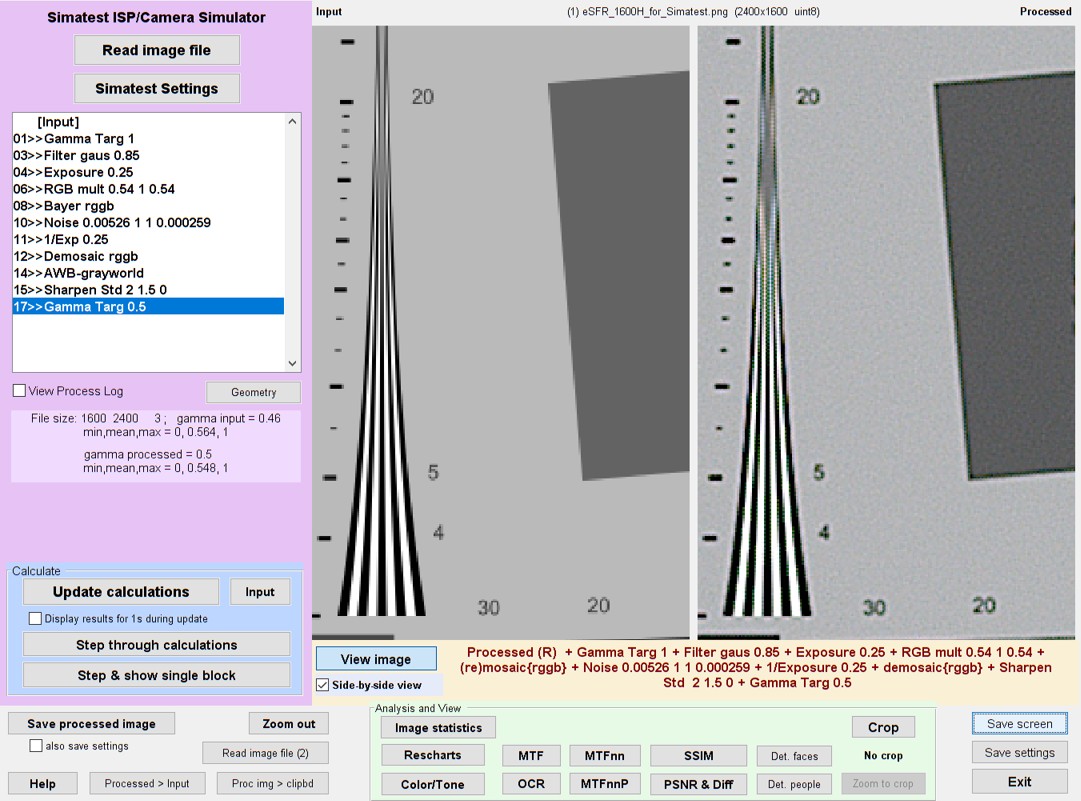 Simatest side-by-side view. Input image on left; processed on right. Zoomed in (for display)
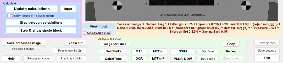
Controls at the bottom of the Simatest window
The Analysis and view (light green) box is listed separately, below. Controls are from left-to-right in column-major order. The View image/processed and Side-by-side view buttons have already been described.
| Save processed image | Save the processed file with the bit depth specified in the light green box in the Settings window. |
| also save settings | (checkbox) Save settings along with the processed image file. |
| Read image file (2) | Read a second image file (into im_processed) for comparison with the original file (which remains in im_input). |
| Proc img > clipbd | Copy the processed image to the clipboard. Unfortunately limited to bit depth = 8. |
| Zoom out | Zoom the image out (display the entire image). This can be helpful when the side-by-side display has framing issues. |
| Processed > input | Move the processed image to the input so that analysis start with the new (formerly processed) image. |
| Help | Open the online Help window. |
| Exit | Bye! |
 Bottom of the Simatest window
Analysis and view controls (in the light green box near the bottom of the Simatest window)
You can select a visual display of the Input or Processed image or a calculated display (an analysis comparing the input and processed images).
| Open the processed file in an external Imatest module. Quick and easy, Used extensively for Simatest Examples. | |
| Image Statistics | Open the image in the Image Statistics module, which can perform cross-section, histogram, and Fourier Transform analysis — and more. |
| Rescharts | MTF (SFR) and other types of analysis, including image information metrics, of the processed image. |
| Color/Tone (Interactive) | Tonal response, noise, and dynamic range analysis for grayscale or color charts in the processed image. Used to calculate Image sensor noise coefficients. |
| Display results inside Simatest. Several compare the input and output. | |
| MTF | Display the MTF (SFR) of the processed / input image as a function of spatial frequency. Sensitive to cropping. |
| MTFnn | Display a polar plot of MTF70-MTF10 of the processed / input image. |
| MTFnnP | Display a polar plot of MTF70P-MTF10P of the processed / input image. |
| SSIM | Display the Structural Similarity Index, of the processed & input images, described on the SSIM page. |
| PSNR & DIff | Display the Peak Signal-to-Noise Ratio and the difference between the processed and input images. |
| OCR | Optical Character Recognition results for the processed image using Matlab’s OCR function |
| Crop | Crops the image for calculations (SSIM, PSNR, and MTF) as well as display. |
| Detect faces & people | Face and people detection using the Matlab CAMShift and detectPeopleACF routines. |
Bottom of the Simatest window
MTF (Modulation Transfer Function; equivalent to Spatial Frequency Response, SFR) is a good example of a Results display. MTF (SFR) calculates the transfer function of the Processed / Input image using a 2D Fourier transform similar to the calculation in the Random module, but with one caveat. Noise should not be added to the simulation if a nice, clean MTF result is required because the 2D MTF calculation is extremely sensitive to noise.
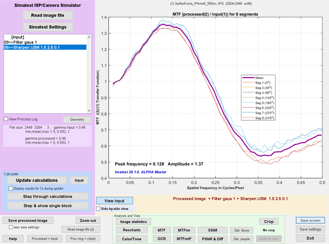 MTF for Gaussian-filtered image with Unsharp Masking
Dropdown menus
Several of the utilities in the dropdown menus at the top of the ISP Simulator window are are duplicates of buttons in the window (intentional redundancy). Highlights (not including duplicates) are
- Display and/or save the Simatest window.
- Save the processed image in one of several formats: standard, pseudo-raw (remosaiced) with several options, monochrome, or HDR.
- Crop the image for MTF, SSIM, etc. analysis.
- Help — Open the instructions and reference web page.
Benefits of Simatest
Now we get to the heart of this post.
The key benefit of using Simatest is that you can predict the performance of an imaging system
- using traditional metrics such as MTF (SFR), noise, SNR, and tonal response,
- as well as the new image information metrics — information capacity, Noise Power Spectrum (NPS), Noise Equivalent Quanta (NEQ), SNRi, and Edge location ,
from properties of the individual camera components, including
- lens sharpness degradation modeled by lens design software (recommended if available; a simple gaussian blur can be used otherwise),
- image sensor noise, calculated from a model based on measurements of raw images or by EMVA 1288 measurements,
- Image Signal Processing (ISP) processing blocks, which can include a large variety of degradations and enhancements.
This enables you to create a “soft prototype” to evaluate how well the combined lens, sensor, and ISP configuration works for the application before building a hardware prototype. This can save a significant amount of time and money. Of course, using Simatest involves a learning curve — it’s not an iPhone — but it should be manageable (we will be developing a set of videos). Once the principles have been learn, getting results from Simatest should be very fast.
Simatest ISP/Camera simulator examples contains several excellent examples showing how Simatest can be used, including
- Modeling, measuring, and simulating image sensor noise,
- Low light performance,
- Simulating sharpness,
- Simulating a camera JPEG image.
We use Low light performance as an example to illustrate how Simatest can be used.
Low light performance
| This section illustrates how to calculate a camera’s key physical properties — image sensor noise coefficients, RGB balance, and approximate lens blur — and use them to predict the camera’s low light (high ISO speed) performance. |
Cameras use two strategies for low light conditions
- Increase the exposure time. This applies primarily to still cameras. Video cameras have limits on their maximum exposure times, typically around 1/30 second, depending on the application. For long exposures, dark current noise, which is measured in units of electrons per second of exposure (e-/s) in EMVA 1288, can be significant. As of April 2025, Imatest does not have a measurement of dark current noise, but it can use EMVA 1288 measurements by substituting iDark in e-/s and exposure time s into \(\displaystyle k_{NDark} = \sqrt{\sigma^2_{Dk}+DSNU^2 + (i_{Dark}\ s)^2} \times \text{Gain}(V/e-) \)
- Increase the analog gain, or equivalently, increase the ISO Speed (Exposure Index). Simatest simulates this by decreasing the signal, adding the image sensor noise, then restoring the signal to its original level.
Strategy for comparing low light measurements with simulations
The tests were performed on a Sony A6000 24 MP Micro Four-Thirds camera with 3.88 μm pixels set to ISO (EI) 100 (the minimum analog gain).
The steps below represent two parallel paths: Odd steps (1, 3, and 5) are measurements; even steps (2, 4, and 6) are the corresponding simulations. The key parameters describing the system, which are determined from the measurement, are
- the image sensor noise coefficients, measured in Color/Tone
- The RGB balance, measured in color/Tone
- The lens/sensor blur, determined iteratively by comparing the measured and simulated MTF curves in (Rescharts) SFR.
Once these parameters have been measured, camera performance can be simulated for a wide variety of conditions. This can save a lot of measurement time.
|
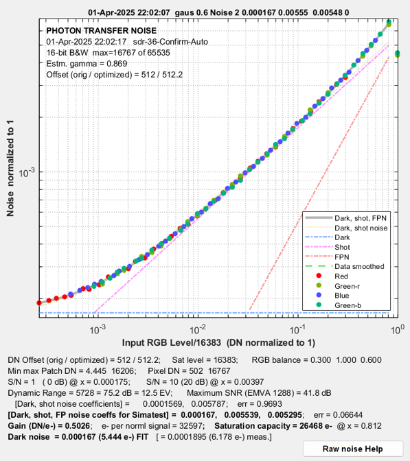
Step 1 – measurement. Photograph a grayscale test chart (preferably a transmissive dynamic range chart), save it in a raw format, then read it without demosaicing into Color/Tone for measuring the image sensor noise coefficients and RGB color balance.
|
|
Step 2 – simulation. Starting with
Run Simatest to simulate the image with noise, then open the simulated image with Color/Tone Interactive, which is very convenient from the Simatest window. The Photon Transfer Curves (PTCs), i.e., noise as a function of digital number, DN, shown on the left and right, below are very close, as expected. |
|
The key settings for calculated by Color/Tone for use in Simatest are noise coefficients, kNdark = 0.0001672, kNshot = 0.005554, kFPN = 0.005477; and RGB (balance) = 0.306, 1.0, 0.606. Simatest settings are shown on the right. The simulation results are on the right, below. The measured and simulated curves are nearly identical. They look slightly different because the x-axis scales are derived from different references:
Click on either image to view full-sized. |
Simatest settings for Color/Tone *Required for characterizing the input image. Not in the ISP Blocks list. |
 A6000 PTC — simulated |
|
Step 3 – measurement. Starting with raw image similar to Step 1 (it can be the same image if it contains a slanted edge for MTF (SFR) measurement), read it with demosaicing into (Rescharts) SFR for measuring the camera MTF (and we also recommend camera information capacity).
|
|
|
Step 4 – simulation. Starting with
Run Simatest. Settings are shown on the right. Then open the simulated image with Rescharts, which is very convenient from the Simatest window. Select SFR, Analyze Image, and note the results for rise distance, information capacities, and MTF50 (shown in the Edge/MTF plot). Adjust the blur sigma (Filter gaus) until the the results are close to the measured values from Step 3. The selected value, Filter gaus 0.55 (σ = 0.55 pixels), is shown in the settings on the right. |
Simatest settings for Rescharts SFR at base ISO speed (100) |
Results for the measured and simulated images are shown on the left and right below. They are very close.
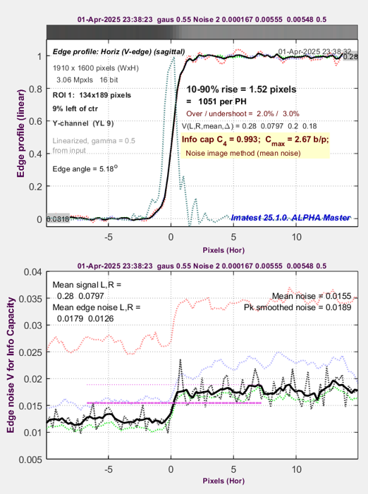
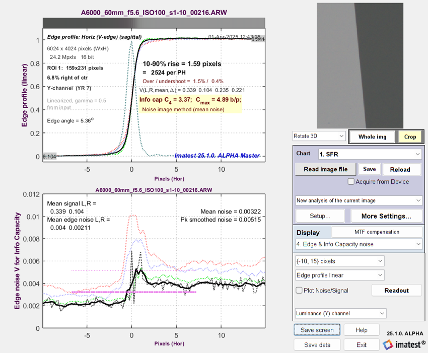 A6000 Edge & Noise plot @ ISO 100 — measured |
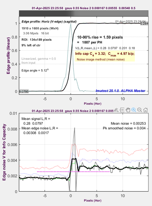 A6000 Edge & Noise @ ISO 100 — simulated |
 Measured (from the Edge/MTF plot) Measured (from the Edge/MTF plot) |
 Simulated (from the Edge/MTF plot) Simulated (from the Edge/MTF plot) |
| Noise is calculated by the MATLAB randn function for each Simatest run. As a result, the noise can look quite different from run-to-run. Here is a different Simatest noise result for the same settings. Little or no peak is expected when there is no Bilateral filtering. | 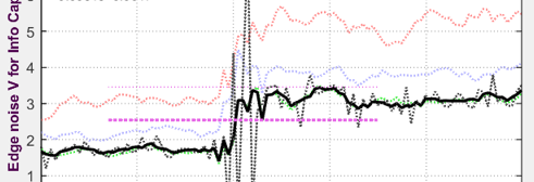 Another run: same settings as above |
|
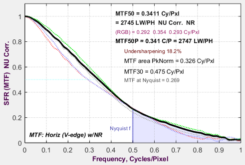
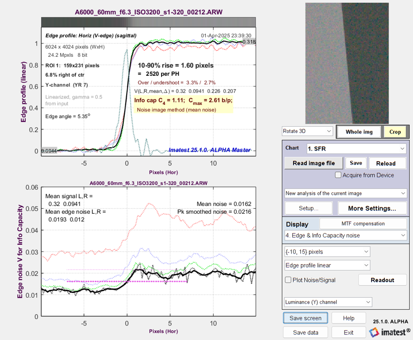
Step 5 – measurement. Repeat Step 3 with just one difference: Increase the Exposure Index to a very high ISO speed (greatly reducing the light reaching the image sensor and compensating by increasing the gain). We chose ISO 3200. The ISO 3200 measurement results (MTF curve, information capacities C4 and Cmax, and spatially-dependent noise) are shown on the left, below. |
|
|
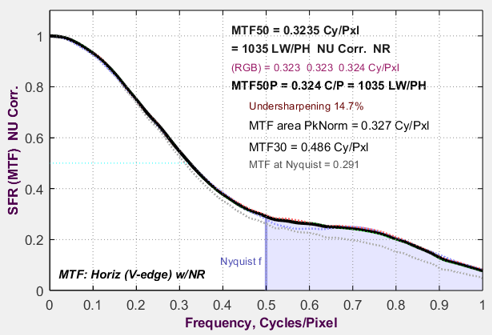
Step 6 – simulation. Identical to Step 4, except two lines, shown in dark red, are added to the Simatest ISP blocks: Exposure and 1/EXP, to simulate high ISO speed (low sensor illumination) by multiplying the signal amplitude by 1/32 before applying noise and 32 afterwards.
The measured and simulated Edge and Noise plots are shown on the left and right, below. They are be very close. |
Simatest settings for Rescharts SFR at ISO 3200 (low light) Two lines added. |
 A6000 Edge & Noise plot @ ISO 3200 — measured |
 A6000 Edge & Noise @ ISO 3200 — simulated |
The simulation is a great success: measured and modeled performance at ISO 3200 are practically spot-on. They are so close, I had to carefully look at the labels above the plots to see which was which.
Appendix
Image sensor noise modelThis section summarizes how to measure image sensor noise to enter into the Simatest Noise block. The full details are in Image Sensor Noise – measurement and modeling. Image sensor noise can be measured with raw (undemosaiced) images or derived from EMVA 1288 measurements. Each pixel in an image file consists of a Digital Number, DN. Simatest works with normalized signal amplitudes, V = DN/DNmax, where DNmax is the maximum digital number supported by the file, typically 2bit depth-1 for demosaiced images, but DNmax is usually different for raw images, where 2ADC precision-1 is common, but not universal. Raw images may have a black level offset, DNoff , described in detail in Image Sensor Noise — Black Level Offset. See Step 5, below. The noise model is \(\sigma_N = \sqrt{k_{Ndark}^2 + k_{Nshot}^2 V + k_{FPN}^2 V^2}\) for linear sensors where the coefficients for dark (read) noise, photon shot noise, and fixed pattern noise, kdark, kshot, and kFPN , are the key parameters of the Simatest image sensor noise model, They are based on James R. Janesick, “Photon Transfer DN → λ”, SPIE Press, 2007, chapter 5, and explained in Image sensor noise model — equations. Noise calculation steps
Noise vs. input pixel level for compact camera with 2.2 μm pixels The numbers to enter into Simatest are shown in the line near the bottom starting with [Dark+shot+FP noise coeffs for Simatest]. Referring to the Noise settings, above, enter Dark noise = 0.000395, Shot noise = 0.009938, and Fixed Pattern noise = 0.006745. RGB balance, which is not part of the noise model, is also an important Simatest input. More details of the calculation for finding dark noise and photon shot noise are in Image Sensor Noise – measurement and modeling. Measured and modeled results are compared in in Simatest Examples. Dark noise is actually a combination of several signal-independent noise sources, described in OnSemi Application Note AND9189/D. Electronic (Johnson) noise is proportional to (4kT)1/2. |