Imatest’s Modified apodization technique reduces noise, making MTF results more consistent, while having a minimal effect on MTF measurements. It works by smoothing the Line Spread Function (LSF; the derivative of the edge) at a distance from the edge center, but not near the center. Because it has little effect on average MTF, it should be kept on unless the result needs to be strictly ISO-compliant. Click on the button below for the full description.
The modified apodization noise reduction technique is available for slanted-edge measurements (SFR, SFRplus, eSFR ISO, SFRreg, and Checkerboard). It can improve measurement consistency for noisy images, especially at high spatial frequencies (f > Nyquist/2), but has little effect on low-noise images. Modified apodization is applied when the MTF noise reduction (modified apodization) checkbox is checked in the Settings windows for any of the slanted-edge modules or in the Rescharts More settings window. ISO standard SFR (lower-left of the window) must be deselected.
Note: Imatest recommends keeping noise reduction (modified apodization) on.
Apodization comes from Comparison of Fourier transform methods for calculating MTF by Joseph D. LaVeigne, Stephen D. Burks, and Brian Nehring, available on the Santa Barbara Infrared website. The fundamental assumption is that all important detail (at least for high spatial frequencies) is close to the edge (Figure 1). The original technique involves setting the Line Spread Function (LSF) to zero beyond a specified distance from the edge. The modified technique strongly smooths (low-pass filters) the LSF instead, which has much less effect on low-frequency response than the original technique and allows tighter boundaries to be set for better noise reduction.
Modified apodization: original noisy averaged Line Spread Function (bottom; green), smoothed (middle; blue), LSF used for MTF (top; red)
Noise reduction algorithm
The Line Spread Function (LSF; derivative of the average edge response; the green curve at the bottom of the figure on the right) is smoothed (lowpass filtered) to create the blue curve in the middle. Smoothing is accomplished by taking the 9-point moving average (the average of 9 adjacent points).
Note: These samples are 4x oversampled as a result of the binning algorithm, so they correspond to approximately two samples in the original image. The smoothing eliminates most response above the Nyquist frequency (0.5 cycles/pixel).
BL and BU are The boundaries (x-axis limits) of the region where the amplitude of the smoothed curve is greater than 20% of the peak value, i.e., the 20% pulse width is the difference between these boundaries.
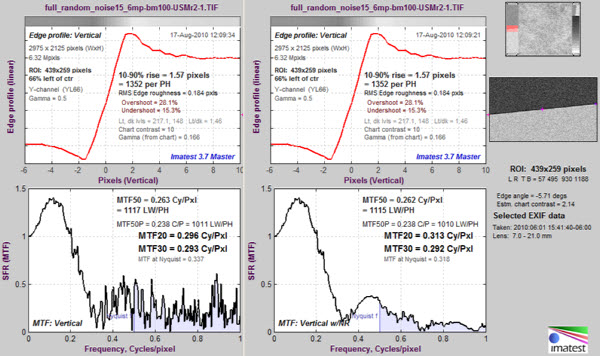
Edge/MTF plot for a noisy image without (L) and with (R) modified apodization noise reduction
PW20 = BU – BL
The apodization boundaries are located at
AL = BL – PW20 – 4 and AU = BU + PW20 + 4 (pixels).
This allows for sufficient “breathing room” so important detail near the edge is unaffected.
The LSF used for calculating MTF is set to the original (unsmoothed) LSF inside the apodization boundaries {AL, AU} and to the smoothed LSF outside, as shown in the red curve above. The benefits of modified apodization noise reduction are shown on the right for an image with strong (simulated) white noise
